Introduction to Economics 2 Dersi 3. Ünite Özet

Introduction

Economists use different models to explain the reasons for these fluctuations in production. However, a common concept lies at the heart of all of these models: Macroeconomic equilibrium. The equilibrium concept mentioned here is the point of equality like supply and demand equality in microeconomics. In other words, equilibrium point shows that there is no tendency to leave once achieved. Macroeconomic equilibrium indicates an economic environment in which income equals aggregate expenditures and there is no tendency to leave this equalization point as far as autonomous expenditures stay constant.

Macroeconomic Equilibrium

In economics, economic equilibrium is the situation where there is no tendency for an economic variable to deviate from this point. In other words, when we talk about equilibrium we refer an economic environment in which economic agents do not change their decisions and behaviors as everything goes planned. This indicates that planned decisions are being made appropriately and that no changes are needed. However, if the planned and actual situation do not match, economic agents will change their behavior and plan to harmonize them. In fact, determination of equilibrium level of income or expenditures is also the process of reaching a situation in which planned and realized are the same.

The approach of the Classical and Keynesian models, which we mentioned before, is different. In the equilibrium approach of the Classical model, thanks to the smooth operation of the market mechanism, the economy is in constant balance, that is, at full employment. The classical model explains the continuous realization of employment in the economy, based on Say’s Law, which states that “every supply creates its own demand”. According to this law, a certain amount of income is generated as a result of the production of goods and services. This income is used again to buy goods and services. Firms purchase or lease the resources required in the production process. They pay their owners in the form of fees, interest, rents, and profits. The amount that the producers pay to the owners of the production factors has to be equal to the value of the goods and services produced. Here, the production factor consumes all the income that the owners have gained and everything produced is sold.

There may be some economic events that cause the failure of Say’s Law. For example, if the production factors want to save money rather than spend a portion of their income, then the all return from productions of the firms will not be expended. Therefore, the quantity demanded for goods and services will be lower than the quantity produced. In case of production or supply surplus, firms will decrease their production and start to lay their workers. This means that the economy diverges from the level of full employment.

According to Keynesian model, equilibrium income can be achieved at the level of underemployment or overemployment. What is important here is the level of aggregate demand. Since it is difficult to change the production capacity that determines aggregate supply in the short term, the level of income depends on aggregate demand or aggregate expenditures. In other words, firms give their production decisions according to the expected aggregate expenditure or aggregate demand level. If the economic units plan to spend more, the sales expectations of the companies will increase and they will make more production. As it is seen, Keynes links the deviations from full employment to the inadequacy of aggregate expenditures in the economy. Accordingly, full employment in the economy can be achieved by an adequate level of aggregate expenditure. Then, Keynesian theory criticizes the views expressed by Classics on investment as a function of the interest rate and on wageprice elasticity. According to Keynesian model, one reason why equilibrium income is not always at full employment level is that investment and saving equality cannot always be provided as Classics argue. The reason for this is that the economic units that save and invest in the economy are generally different from each other. These economic units give savings and investment decisions for different reasons.

Determination of Equilibrium Income Level

Equilibrium level of income in the economy means that aggregate supply and aggregate demand are equal to each other. Aggregate supply refers to the amount of goods and services that are desired to be produced in the economy. At the same time, income from the sale of these goods and services is national income. Aggregate demand represents the level of expenditure that economic units are planning to make at various income levels. Therefore, the determination of equilibrium income and expenditure level for an economy is the period of determining the level of income and expenditure, which is equal to what is planned and realized.

Keynesian economy argues that equilibrium level of income is realized at the level where aggregate demand equals aggregate supply. Since the economy’s short-term production capacity is difficult to change in the short-run, the effective factor that determines the short-run equilibrium level of income is aggregate demand. Aggregate demand is called effective aggregate demand, at the level where the aggregate demand is equal to the aggregate supply.

We can use the aggregate expenditure function to analyze how the level of equilibrium income is achieved. Aggregate demand is shown here as the aggregate expenditure function. The aggregate expenditure function gives us the value of aggregate expenditures planned at different income levels. The actual expenditures in the economy are always equal to the income and the production. These expenditures include stock variables. Depending on stock changes, investments automatically increase or decrease, so actual expenditures is always equal to income, production or, GDP. Equilibrium GDP Level is the level at which planned aggregate expenditures are equal to GDP.

Another way of determining the level of equilibrium income of the economy is to examine leakages and injections in the income-expenditure flow. This improved analysis of the savings-investment equation shows that if the total leakages are equal to the total injections, incomeexpenditure equality is achieved and the level of equilibrium income is reached.

Leakages are used to denote reductions in autonomous components of aggregate expenditures. It is possible to mention three types of leakages from the incomeexpenditure flow:

• savings
• taxes
• imports

In order to achieve equilibrium in the economy, the leakages from income – expenditure flow must be balanced by additions (i.e., injections) to this flow. Injections are additions to income-expenditure flow.

There are three types of injections for income-expenditure model:

• investments
• government expenditures
• exports

When the households decide to increase their savings without a change in income level, interesting contradiction called as saving paradox will arise. Saving paradox is the reduction in the consumption expenditures and, therefore, income because of rising savings.

If the increased savings can be turned into investment expenditure, no problems arise. Only when the increased savings are not “injected” into the economy, the emergence of the saving paradox is possible in the economy. In other words, increasing savings in the economy will cause total spending and income to decrease as long as it does not turn into investment. Therefore, it is very difficult for the saving paradox to emerge in real life.

Changes in Equilibrium Income and Expenditure Level

We have defined the equilibrium point in the economy as the point at which there is no tendency to leave. But this equilibrium point itself has a tendency to change due to the dynamics of the economy. For example, the level of equilibrium GDP can move to a lower or higher level than in the initial state over time, and may be in equilibrium at this new point. When we increase the autonomous expenditures, which vary independently from the income, we can also increase the equilibrium level of GDP.

The multiplier is a coefficient that can give us to opportunity to calculate how much income will change when there is a shift in aggregate expenditures, stemming from the change in autonomous expenditures. The multiplier value is always greater than 1. The reason for this is that the change in autonomous expenditure leads to an additional change in consumption expenditures. Here, the determinant of the size of the effect is marginal propensity to consume. As you remember, the marginal propensity to consume gives us how consumption rises when income rises. For example, the primary effect of 1 unit increase in autonomous expenditure would be to increase production and income by 1 unit. If the marginal propensity to consume is large, this increase in income leads to a large increase in consumption. In this case the multiplier effect will also be large. If the marginal propensity to consume is small, this increase will lead to a low change in consumption. In this case, the multiplier effect will be small. As the change in consumption expenditure is determined by the marginal propensity to consume, the increase in consumption expenditure of unemployment benefit earners will be equal to the change in the current amount multiplied by the marginal propensity to consume (MPC). Some of the current increase will be attributed to savings depending on the marginal propensity to save (MPS). The increase in import spending will be equal to the marginal propensity to import (MPI) multiplied by the income increase. These leakages are determined by marginal propensity to save (MPS) and marginal propensity to import (MPI):

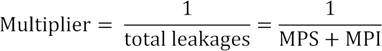
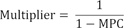
The rest of the income increase after separating leakages is devoted to domestically produced goods and services, and the ratio of this amount to income increases is measured by marginal propensity to consume (MPC). Therefore, we can also calculate the multiplier by writing the same formula in terms of MPC:

Multiplier is a useful tool for assessing the impact of changes in economic policies on the economy since it helps to calculate and analyze the effects of a change in autonomous expenditures on GDP.

Full employment level of income is the level of income that will be attained in the economy if all the factors of production participate most effectively into the production. This level of income is called potential GDP. If the economy is below the full employment level, some of the production factors will remain idle. This is the level of underemployment equilibrium.

The negative difference between the actual GDP and the potential GDP in an economy is the negative GDP gap or deflationary gap. Deflationary gap is the expenditure gap when the economy is in equilibrium below the full employment level of income.

An increase in the expenditures in an economy causes the income level to rise. This will take place in real terms up to full employment level and in nominal terms after full employment level. If expenditures still go on to increase, only the nominal income may increase. Inflationary gap is the excess of expenditures when the economy is in equilibrium above the full employment level of income.