Mathematics 1 Dersi 8. Ünite Özet
Multivariable Functions
What is a multivariable function?
When a quantity depends on more than one variable, we refer to it as a function of several variables or a multivariable function.
For example, in case of two variables a function of two variables z = f ( x , y ) is defined, if for each ordered pair ( x , y ) belonging to a set A ? R 2 , there is a uniquely defined real number z ? R . Then A is called the domain of the function f : A › R . Elementary examples of multivariable functions may be given as f : A ? R 2 › R , f ( x , y ) = x 2 + 2 y 2 - xy , or g : A ? R 3 › R , g ( x , y ) =  . Although the domain is not specified but given as a set A , it is clear from the definition of both functions that they are defined over all R 2 and R 3, respectively.
The graph of function defined on a set A ? R may be represented in 3 dimensions. Such an example is, say, 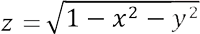 , which corresponds to the upper sphere with centre the origin and radius 1. However, when the function is defined on a set A ? Rn , where n ? 3, then we cannot represent the graph since the graph of such functions will be on the 4-dimensional space.
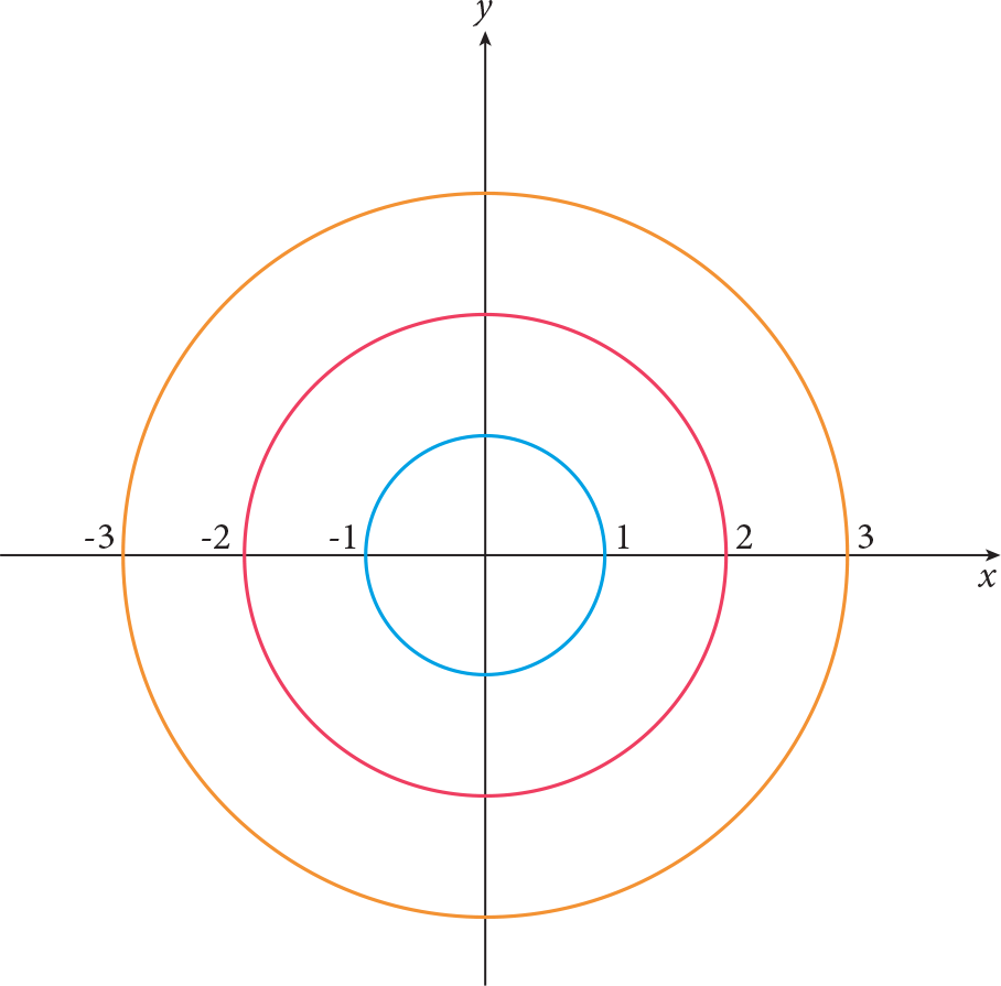
A 2D representation of the 3D graph may be shown through contour lines which are plotted in ( x , y ) coordinate frame and are given by z =const. By choosing different values of the constant on the right-hand side of this equation, we obtain different cross sections of the surface on different horizontal planes. One such example is the cross sections of the sphere with centre origin given below:
Limits and Continuity
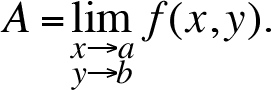
The idea of limit of a function of one variable may easily be extended to functions of several variables. However, in the case of even two variables the direction of approach to a point for which the limit is being sought for is inredibly varied. In the single variable case we approach a point either from left or from right, whereas in higher dimensions this aprroach is arbitrarily many. Although the definition of limit stays the same due to the variedness of the aprroach actaul calculations are much harder. Now, let us define the limit:
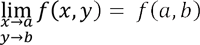
For a function of two variables y = f ( x , y ) we define a real number A as a limit at the point ( x , y ) = ( a , b ) if for any positive value  , it is always possible to find such value
  , such that for all ( x , y ) satisfying
 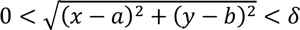 , the values of the function satisfy the condition | f ( x ) - A |< .Then we write
 .
.
Continuity of a multivariable function is defined similarly to that of a function of one variable. For example, in case of two variables we shall define the function z = f ( x , y ) to be continuous at the point (a, b) if,
- the function z=f (x, y) is defined at (a, b)
- the limit of the function z=f (x, y) at (a, b) exists
- and this limit coincides with the value of the function,i.e.
In many cases readers get confused about the continuity of the functions like f ( x , y ) = 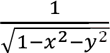 when x 2 + y 2 = 1, i.e. when the denominator is zero. But, according to (i) above, the function must be defined at a point in order to talk about its continuity. Since, here, the function is not defined on the unit circle, we do not consider its continuity at these points. For the remaining of the points where the function is defined, i.e. inside the unit disk, the function is obviously continuous since its limit value and the function value at every point inside the disk is the same.
Partial Derivatives
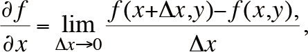
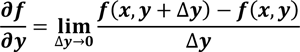
As we have already mentioned the approach to a given point in n-dimensional space is unlimited which makes the limit much harder than its one-dimensional counterpart. Since, the derivative is not defined through limits, the concept of derivative is quite demanding in higher dimensions. However, there are certain types of differentiation in higher dimensions one of which is partial derivatives. This concept takes advantage of the derivative of a function of single variable. Let us define it for functions of two variables, i.e. f ( x , y ). For a function z=f (x, y) of two variables we have two first order partial derivatives
and
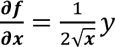
Note that differentiation along, say, variable x means that the other variable is “frozen”, i.e. treated as a constant. This makes differentiation quite straightforward just as the differentiation in the one variable case. As an example, let us calculate the partial derivatives of f ( x , y ) = ? x / y :
 and
and 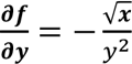 . In the first one we calculated the derivative of the square root function taking y as a constant, and in the second one we differentiated 1/ y and considered ? x as a constant.
The usual rules for single variable differentiation also applies for the multivariable functions (see Chapter 6). It must be kept in mind, however, that the partial derivatives do not correspond to the derivative of a multivariable function but only to derivative along the coordinate axes.
Tangent plane and normal line to a surface
Let us remember that the equation of a tangent line to the graph of a function y=f(x) at a point x=a is usually written as
y = f ( a ) + f '( a )( x - a ).
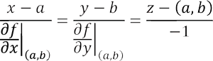
In the case of a function of two variables, say for notational convenience, z = f ( x , y ) , the equation of the tangent plane around the point ( x , y ) = ( a , b ) to the graph of z is given by
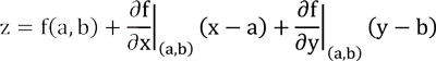
As follows from the last equation, the vector with coordinates 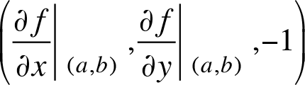 will be perpendicular or normal to this tangent plane. Then the equation of a normal line, passing through the point (a, b, f (a, b)) perpendicular to the tangent plane, is
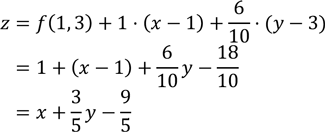
We may calculate the tangent plane to the graph of f ( x , y ) = x log(1 + y 2 ) at the point (1,3). To this end we calculate the partial derivative which are
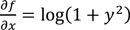 and
and  The values of partial derivatives at (1,3) are, respectively, 1 and 6/10 . The tangent plane, then, is
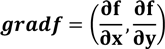
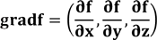
The gradient
The gradient of the function is introduced as a vector, the components of which are the associated partial derivatives, i.e. for a function of two variables z = f ( x , y ) the gradient is
Clearly, in case of a function of three variables u = f ( x , y , z ) the gradient is
One of the most important properties of the gradient is it is perpendicular to the contour lines of the function, which also implies that the gradient vector is normal to the tangent plane of the surface at the point in question.
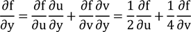
Change of variable. Chain rule
Chain rule, like its counterpart in one variable, is a rule for calculating the partial derivatives of composite functions, i.e. functions of functions. Assume that
z = f(x, y) = f ( x(u, v), y(u, v) ) = F(u, v).
So, f is a function of (x, y) and x and y are functions of (u, v). So, the chain rule is stated in the following way:
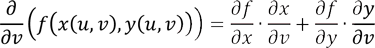
and, similarly,
In this context, changing variables means that writing the variables as functions of new variables. Consider the following example:
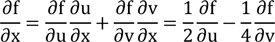
Write the differential equation 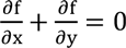 in the new variablesu = (x + y)/2and v = (y - x)/4. If we calculate
  we find
and
So, inserting back into the original equation we find
Note that with the change of variable we now have a much simpler equation (differential) which may be solved easily (for this we have to wait until the second book).
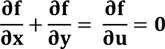
Local extrema of multivariable functions
In functions of one variable we encountered local extrema of functions being local minimum or local maximum points and/or values. In case of multivariable functions, the situation is slightly more complicated with the introduction of one more type of point, namely the saddle point. The function’s behaviour around such points is, in a sense, indeterminate. Departing from this point and moving in an arbitrary direction the function may either decrease or increase and therefore it neither defines a minimum or a maximum. We give now a test for determining the extremum points of a function.
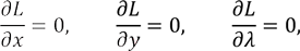
First, we need to find stationary points by solving simultaneous equations 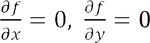
Then, for a given stationary point P, one needs to evaluate
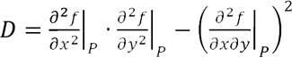
Then, if D > 0 and 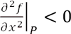 , P is a point of a local minimum.
If D < 0 and , then P is a point of a local maximum.
If D < 0, then P is a saddle point.
Restricted local extrema of multivariable functions
Local extrema of functions are used to solve optimization problems such as increasing the profit of a company, reducing the costs depending on the raw materials, etc. In some cases, we have to impose constraints on the optimization problems we consider. Below we consider in detail the case of a function of two variables. Then, there is usually just one restriction, so the formulation of the problem looks as follows
z = f ( x , y ) › extr
g ( x , y ) = 0
Here z = f ( x , y ) is often referred as the objective function, and g ( x , y ) = 0 is a constraint. The simplest approach to the problem is possible when one of the variables may be expressed in terms of the other from the constraint, then the problem reduces to standard extrema problem for a function of one variable. Let us reproduce here the example from our book to analyse the approach in detail.
A rectangular camping area of area 2592 m 2 needs to be designed. The area is bounded from one side by the forest and requires fencing from the other three parts (one length and two widths). Find the optimal length and width in order to have minimal length of the fencing required.
Solution:
Let x and y be length and width of the designed camping area, respectively. Then the objective function, the fencing length is f ( x , y ) = x + 2 y . The constraint of the area being 2592 m 2 is written as xy = 2592 or xy - 2592 = 0. Hence, the Lagrangian formulation is given by
L ( x , y ,  ) = x + 2 y + ( xy - 2592).
Let us find the stationary points of this function. Then,
which gives
1 + y = 0, 2 + x= 0, xy - 2592 = 0.
Eliminating from the first two equations, we have (clearly both x and y are not zero in view of the constraint)
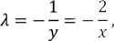
hence x = 2 y , so from the constraint 2 y 2 = 2596 , therefore y = 36, x = 72, and the sought for length of the fence is 72 + 36 + 36 = 144 m.
-
Çıkmış Soruları Gönder Para Kazan!
date_range 2 Temmuz 2026 Perşembe comment 25 visibility 4665
-
2025-2026 Öğretim Yılı Yaz Okulu Kayıt Duyurusu
date_range 29 Haziran 2026 Pazartesi comment 4 visibility 977
-
2025-2026 Öğretim Yılı Bahar Dönemi Dönem Sonu (Final) Sınavı Sonuçları Açıklandı!
date_range 18 Mayıs 2026 Pazartesi comment 1 visibility 3157
-
AÖF 2025-2026 Öğretim Yılı Bahar Dönemi Dönem Sonu Sınavı sorularına itiraz
date_range 12 Mayıs 2026 Salı comment 1 visibility 1357
-
2025-2026 Bahar Dönemi Dönem Sonu (Final) Sınavı Sınav Bilgilendirmesi
date_range 4 Mayıs 2026 Pazartesi comment 2 visibility 3295
-
Başarı notu nedir, nasıl hesaplanıyor? Görüntüleme : 28037
-
Bütünleme sınavı neden yapılmamaktadır? Görüntüleme : 16404
-
Harf notlarının anlamları nedir? Görüntüleme : 14809
-
Akademik durum neyi ifade ediyor? Görüntüleme : 13935
-
Akademik yetersizlik uyarısı ne anlama gelmektedir? Görüntüleme : 11855