Mathematics 1 Dersi 7. Ünite Özet

Supply and Demand

Two essential concepts of economics are the supply and demand. Supply, in the simplest terms, is the amount of a product that is available to the customers. Demand, on the other hand, is the willingness of people to buy a certain product. In many problems of economics modelling of supply and demand may be achieved through the use of linear functions, i.e., functions of the form f(x) = ax + b Therefore, it is necessary to understand the notion of a line and its certain properties such as its slope, and its intercepts of the axis in the plane.

Depending on the slopes of the lines for supply and demand, we observe that for a given commodity the market may show different attitudes: there may be a high demand for the product, or there may be a high supply than necessary. The point of equilibrium where the supply and demand curves intersect tells us that the demand for a product is equal to its supply. Knowing this point may help companies to decide how many units of a product they should produce.

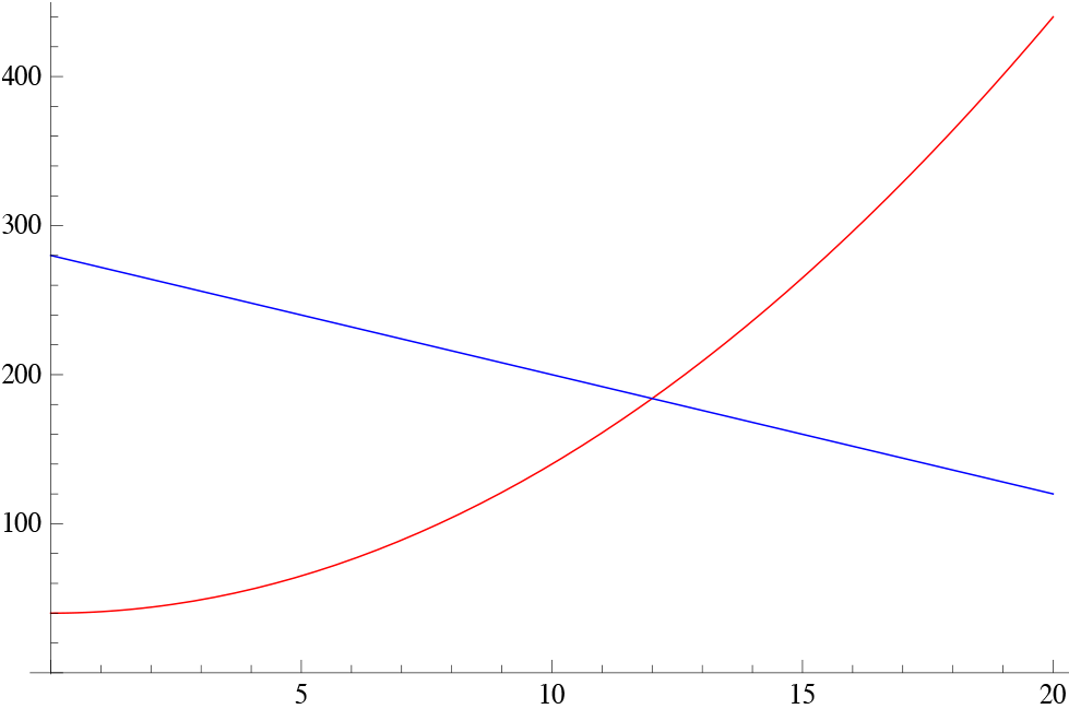
We may consider, for example, a company supplies x units of a particular product to the market when the price is p = S(x) liras per unit, and the same number of units will be demanded by the customers when the price is p = D(x) liras per item. Let us assume that the functions S(x) and D(x) are given by S(x) = x ² + 40 and D(x) = 280 - 8 x . The first question we may ask is when the market achieves equilibrium; in other words, at what level of production and the price of the product the supply and demand become equal. If we equate, therefore, the supply and demand curves we get

x ² + 40 = 280 - 8 x ? x ² + 8 x - 240

The solution is easily found as x = -20 and x = 12. Since the price cannot be negative we find that the market is in equilibrium when x = 12. We may see the graph here. The red graph is the supply curve and the blue graph is the demand curve. The intersection point is the equilibrium point. To the left of this point there is surplus in the market where to the right, there is a shortage in the market.

Break-even Analysis

It is important to know the cost of producing a commodity, so that the revenue and therefore the profit may roughly be calculated before the production. e costs are divided into two: fixed costs and variable costs . If the fixed cost of a product is denoted by a and its unit variable cost is denoted by v, then the total cost function is

C(x) = vx + a

The total revenue function is defined as the product of items sold, say x , and the price per unit item, p , so that

R(x) = px.

Now, if a company neither loses any money nor gains any profit from the sale of a commodity, it is said that the company has broken even . To find the point where breakeven occurs one only needs to equate the total cost to the total revenue, and find the value of x .

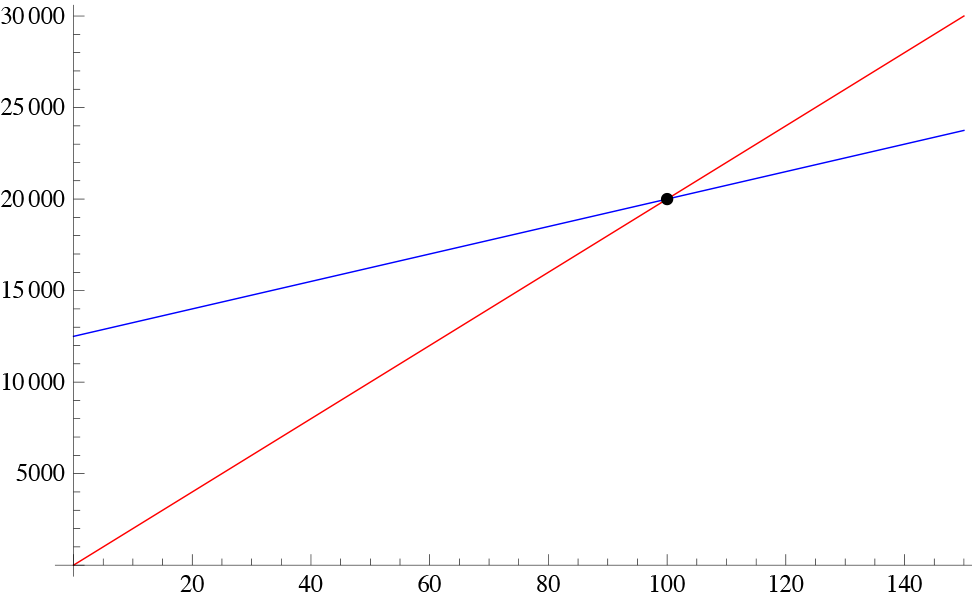
As an example, let us investigate a hardware manufacturer who sells hard drives for 200TL per unit. The fixed cost of the company is 12500TL and the cost of production of one unit of hard drive is 75TL. In this case, the revenue function is R(x) = 200 x and the cost function is C(x) = 12500 + 75 x . In order for the company to break even these functions must be equal which is written as 200 x = 12500 + 75 x , from which we deduce x = 100, i.e. the company must produce at least 100 drives just to break-even and any production above this quantity will turn into profit. In the figure below, red is the revenue function whereas the blue is the cost. The point of intersection is the break-even point.

Marginal Analysis

Derivative is defined as the rate of change of a certain quantity with respect to another quantity. In economics, it is important to determine the change in a quantity (product, price, etc.) that results from a 1 unit increase in the production. This change approximately corresponds to the derivative of the quantity in question and it is called as the marginal change, actually meaning the derivative. Quantities such as cost, revenue, and profit may be investigated through the use of derivatives and in economics this is called as the marginal analysis.

As the derivative is a measure of change in a given quantity, it may be employed to determine the minimum or maximum values of functions. This proves to be very useful in economics since many economical terms may be expressed in terms of mathematical functions. We define the marginal cost, marginal revenue and marginal profit as the derivative of the total cost, total revenue, and the profit functions. So, in order to make the profit of a company maximum all we need to do is use the derivative to find the point, i.e. the amount of the product to be produced, which makes the profit function maximum.
Let us assume that a shoe manufacturer’s profit function is P(x) = -0,05x ³ + 0,07x ² + 25x - 150 , where x denotes the number of shoes to be produced. The marginal profit function is the derivative of the profit function which is P'(x) = -0,15x ² + 0,14x + 25 . If, for example, the numbers produced is x = 10 then the marginal profit is P'(10) = . For x = 50 we get P'(50) = -343, and for x = 70 , P'(70) ? -700 . It is clear that as the manufacturer increases the number of production there is a serious loss in the profit, which may be due to various factors such as demand or production costs.

Elasticity

In economics, the term elasticity refers to the sensitivity (responsiveness) of one economic variable to changes in another economic variable. In order to prevent the use of dimensions, it is measured as the ratio of percentage changes , rather than absolute changes. We define the price elasticity of demand as

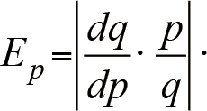
The price elasticity of demand may be classified as inelastic (E _p < 1 ), unit elastic (E _p = 1 ), and elastic (E _p > 1). In the first case the consumers are said to be unresponsive to a change in price; in the second case the change in price and demand are the same and in the third case the consumers are very sensitive to the changes in price.

The effect of price elasticity of demand on the revenue may be classified as follows:

a. If demand is elastic, i.e. | E _p |>1, revenue R (p) = p · q(p) decreases as price p increases.
b. If demand is inelastic, i.e. | E _p |<1, revenue R increases as price p increases.
c. If demand is of unit elasticity, i.e. | E _p |=1, revenue is unaffected by a small change in price.