Mathematics 1 Dersi 5. Ünite Özet

Limits of Functions

The limit concept is at the heart of differential and integral calculus and it is the aim of this chapter to introduce the limit concept and define the limits of functions. Limit is the number which the value of a function “approaches” as its argument (variable) approaches to a certain point. In this context “approach” means that as the variable gets arbitrarily close to a particular point, but never reaches it, the function f may get sufficiently close to a certain value, say L . Since, what is important is the behaviour of the function f around this particular point, say x ₀ , the value of the function at x ₀ is irrelevant to the limit concept. Therefore, the definition of the limit of the function f at a given point x ₀ is that f(x) can be chosen arbitrarily close to a number L by taking x sufficiently close to x ₀ , but not equal to x ₀ . We then say that the limit of f as x approaches x ₀ is L and we write it as

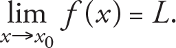
where x › x ₀ indicates that x approaches the point x ₀ . We read 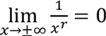as '' The limit of f as x approaches x ₀ is L ''. Thus, if there is such value L, f(x) may not be defined at the point x ₀ , we can make the value of f(x ) as close as we want to L . In other words, the limit of a function at a given point x ₀ determines the behaviour of the function near x ₀ .

To understand this concept, we want to determine the behaviour of f(x) = x ² around the point x = 2. That is, what does the value f(x) approach when x tends to the point x = 2? Now, let us consider points x around x = 2 such that the distance between points x and x = 2 gets smaLer as seen in the Table below.

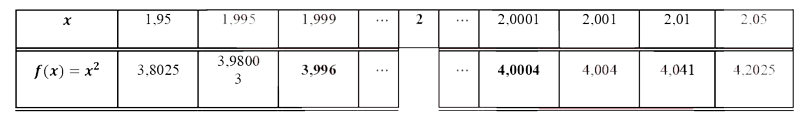
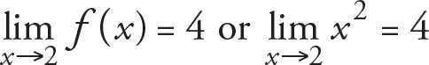
In this case, from the table given above, as the numbers x get closer and closer to the point 2 (either with smaLer or greater values than 2), since the value f(x) appear to be sufficiently close to the value 4, we estimate that limit is 4 and we say that 4 is the limit of the function f(x) = x ² as x approaches the point x = 2 . In mathematical notation, this statement is written in the form

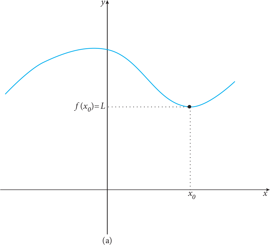
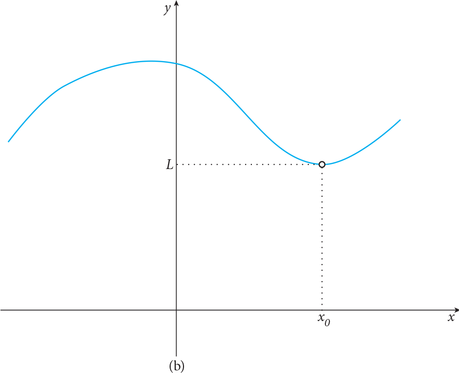
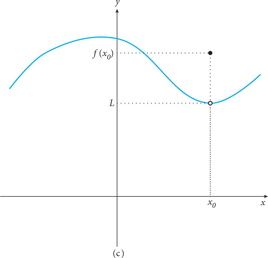
If ,  the following figures explain there will only be three different cases. In the first one, f(x ₀ ) = L , i.e. the function is defined at x = x ₀ and has the same value as its limit; in the second case, f(x ₀ ) is not defined but it has a limit value; in the last one, the function is defined but the value of f is different than its limit value, i.e. f(x ₀ ) ? L .

One –Sided Limits

Although a function may have a limit at a given point, it is sometimes enough to know the behaviour of the function to the right or left of a point x ₀ . In this step, we just need to consider the approach of x to the point x ₀ from only one side.

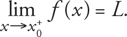
If the approach is from one-side, say from the right of x ₀ , we use the notation x › x ₀ ⁺ ; if it is from the left of x ₀ , we use the notation x › x ₀ ^- . In the case, we say that the right limit of f is L and it is denoted by

,

and that the left limit of f ( x ) is L and this is denoted by

respectively. Note that there is important relationship between two-sided and one-sided limits and this relationship can be given as follows:

if only if and

Now, we consider two significant examples which we wiL frequently be used to calculate the limits of various functions:

Consider the constant function f(x) = c , where c ? R . For any x ₀ ? R ,

Let f(x) = x be the unit function and x ₀ ? R . For this function, we have

Rules for Calculating Limits

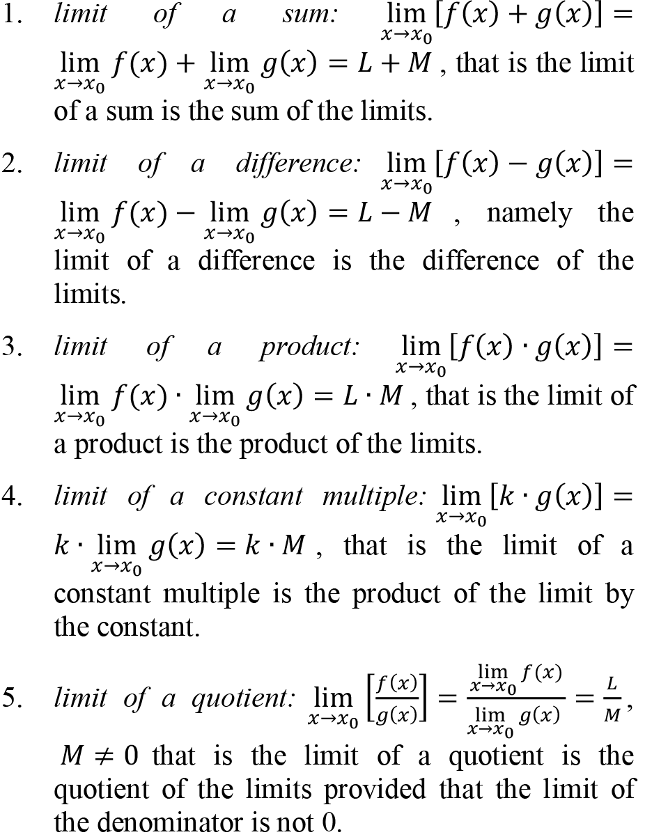
Now, we give the following properties of limits which make it easy to calculate limits of the functions encountered in this chapter provided that the limits of elementary functions are known.

Limit rules:

Suppose that k is a constant and the limits , exist and are L and M , respectively. Then

Note that limit rules are applicable to one sided limits by the symbolism x › x ₀ can be replaced by x › x ₀ ⁺ or x › x ₀ ^- .

Infinite Limits and Limits at Infinity

Now, we are going to extend the idea of limit. We will consider limits involving the concept of infinity. We employ the symbols -? and ? to indicate that either a variable or a quantity unboundedly grows in the negative and positive direction, respectively. We will consider two kinds of limits:

• infinite limits
• limits at infinity

Let f be a function defined about the point x ₀ , except possibly at x ₀ itself. If f(x) takes arbitrarily large values ( f(x) increases without bound) as x approaches x ₀ then we say that the limit of f as x approaches x ₀ , is infinity . It is denoted symbolically by

In a very similar manner, we have the following: if, as x approaches x ₀ , f(x) takes arbitrarily large negative values , i.e. f(x) increases without bound in the negative direction, then we say that the limit of f as x approaches x ₀ , is minus infinity and denote it symbolically by

Similarly, by making use of the limit introduced here, we may answer the interesting question:

“How does a function f behave as its variable x become arbitrarily large, i.e. what happens to f as x › -? or x › +?” ?

Symbolically we write and say that the limit of f(x) is L , if it exists , as x approaches infinity or negative infinity . Such a number L may not exist which indicates that f approaches +? or -?.

Recall that the symbols -? and ? do not represent numbers . Actually, they imply unbounded behaviour when used in the limit concept.

Note that if the function is a polynomial the term with the highest degree of the polynomial determines its behaviour. That is, the term with the highest degree dominates the remaining terms as x becomes large. Also, the limit which is expressed as ( r ? Q , provided that makes sense ) is always true.

Continuity

Finally, the continuity of a function which is a farreaching and important concept in calculus is shortly discussed. Using the limit, we define the continuity of a function through the point x ₀ can be drawn without lifting the pencil from the paper.

Finally, the continuity of a function which is a farreaching and important concept in calculus is shortly discussed. Using the limit, we define the continuity of a function f at a given point.

A function f is called continuou s at the point x ₀ if

Note that if f is continuous at the point x ₀ , the following three conditions must be ensured:

• f(x ₀ ) is defined, that is, x ₀ is in domain of f ,
• exists,
• 

Thus, the graph of a continuous function at a given point x ₀ of its domain has no breaks , holes, or jumps at this point; in other words, the graph of a continuous function through the point x ₀ can be drawn without lifting the pencil from the paper.

Note that, despite a function f may not have a limit at x ₀ in its domain, it can still have one-sided limits at x ₀ (that is, the function f may have a jump at x ₀ ). Thus, in this case, we can extend the definition of continuity:

If , we say that f is right continuous at x ₀ and if , we say that f is left continuous at x ₀ .

Now we can give a relation between continuity and onesided continuity of a function f in the following manner:

A function f is continuous at x ₀ if only if it is right and left continuous at this point.

If f is not continuous at x ₀ or if f is not defined, we say that f is discontinuous at x ₀ . That is, if any one of the three conditions listed above are not satisfied, then f is said to be discontinuous at x ₀ .

In the case of complicated functions (sums, quotients, composite, etc.) we can make use of the properties of limits (see, Limit Rules ) to give significant properties that may help us determine the continuity of given functions. That is if the functions f and g are continuous at a point x ₀ , then the sum f + g, the difference f - g , the product f • g and the quotient (provided that g(x ₀ ) ? 0 ) are continuous at x ₀ .

Significant properties of continuous functions mentioned in this chapter is that if a function f is continuous on the closed, bounded interval [ a, b ] must have an absolute maximum value and an absolute minimum value on the interval [ a, b ].