Mathematics 1 Dersi 3. Ünite Özet

Introduction

Chapter 2 the concept of functions was introduced. In this chapter we focus on polynomial functions which are a special subset of functions. Specifically, we will introduce the first and the second-degree polynomial functions of a single variable. Many real-world situations can be explained through using polynomial functions. Polynomial functions are widely used in different areas of science such as business, medicine, psychology, and sociology.

Polynomials

We shall be mainly concerned with two types of functions, namely linear and quadratic functions, which belong to a much larger class of functions called polynomials. First we give the general definition of polynomials.

A polynomial function of degree n is a function f : R ? R of the form

f(x) = a _n x ⁿ + a _n - ₁ x ^n-1 + ... + a ₂ x ² + a ₁ x + a ₀

where a _0, a _1, … ,a _n are real numbers, n is a natural number and a _n ? 0.

The form

f(x) = a _n x ⁿ + a _n-1 x ^n-1 + ... + a ₂ x ² + a ₁ x + a ₀

for a polynomial was first used by the French philosopher and mathematician Rene Descartes.

The degree n of a polynomial in one variable is the greatest exponent of its variable. The numbers

a _n ,a _n-1 , ... ,a2      a ₁ ,a ₀

are called the coefficients of the polynomial. The leading coefficient a _n is the coefficient of the term with the highest degree. If a _n = 1 , the polynomial function is called a monic polynomial. The number a ₀ is the constant coefficient or constant term.

If f(x) = a ₀ and a ₀ ? 0, we say the degree of f is 0. If f(x) = 0 , we say f has no degree. However, some authors prefer to say that its degree is undefined. If f(x) = a ₀ , it is called a constant function.

Polynomial equations

We have defined a polynomial function of n ^th degree as a sum

f(x) = a _n x ⁿ + a _n-1 x ^n-1 + ... + a ₂ x ² + a ₁ x + a0

If f(x) = 0 then its called a polynomial equation. Therefore, the polynomial equations are equations of the form

a _n x ⁿ + a _n-1 x ^n-1 + ... + a ₂ x ² + a ₁ x + a ₀ = 0

Suppose that f(x) is a polynomial equation of degree 1. We may, hence, write it as

f(x) = ax + b = 0

where a and b are real numbers and a ? 0 . This equation is called a linear equation in one variable.

Let f be a polynomial function. If f(x ₀ ) = 0 for x ₀ ? R, then x ₀ is called a root of the polynomial function. The set {x ₀ : f(x ₀ ) = 0} is called a solution set.

Suppose that f( x ) is a polynomial equation of degree 2. We may write it as

f(x) = ax2 + bx + c  = 0

where a , b and c are real numbers and a ? 0 . This equation is called a quadratic equation in one variable.

Let us consider the quadratic function f(x) = x ² + 1 . We want to find a solution of f(x) = 0, i.e. we want to find the number x which, when inserted in the function, will give zero. f(x) = 0 means that x ² + 1 = 0. So, x ² = -1 . But we know that the square of any real number is non negative. Therefore, there is no solution. For this reason, the solution set is empty set. We can show it as { } or Ø.

Suppose that ax ² + bx + c = 0, a ? 0 . We would like to construct a formula to find the roots of this quadratic equation. We can re-write the equation factoring out the GCF (greatest common factor).

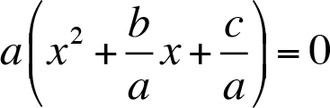
We know that “ ıf a * b = 0 then a = 0 or b = 0 for all a, b ? R”. So,

Let us use the identities given above

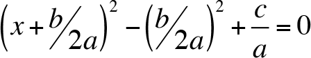
Thus,

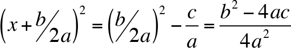
Apply the square root property,

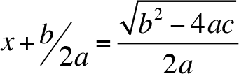
and

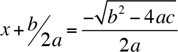
Finally,

and

We can write this formula (quadratic formula) in short as

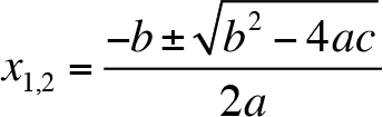
In the quadratic formula, b ² -  4ac is called the discriminant of the quadratic equation and we use the symbol ? (capital Greek delta) for discriminant:

?= b ² - 4ac

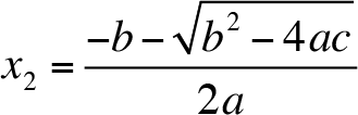
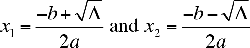
If the discriminant is positive, then there are two distinct roots. Both roots are real numbers and they are given by

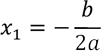
If the discriminant is zero, then there is exactly one real root. It is sometimes called a double root. It is written as

If the discriminant is negative, then there are no real roots.

In general, let x ₁ and x ₂ be any two real numbers which are roots of a quadratic polynomial. This means that,
x - x ₁ = 0 and x - x ₂ = 0 . Thus, (x - x ₁ ) (x - x ₂ ) = 0 .
On expanding the product, we arrive at

x ² - (x ₁ + x ₂ )x + (x _{1 .} x ₂ )  = 0 .

The general form of a quadratic polynomial is

ax ² + bx + c = 0 .

If we divide both sides by a , the polynomial becomes a monic polynomial which is

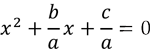
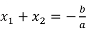
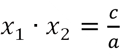
We observe, from the expansion above, that the sum of the roots of the polynomial is equal to and their product is That means,

and

Graphs of Polynomial Functions

Up until this part we defined polynomial functions and discussed their basic properties. We investigated the “roots” of first and second degree polynomials called linear and quadratic functions, respectively. In this part we investigate the graphs of polynomial functions. Let f(x) be any polynomial function. For any real number x , (x, f(x)) is called an ordered pair.

The graph of a function f is the collection of all ordered pairs. The graph is drawn on the Cartesian coordinate system. So, the graph has two dimensions.

Let f(x) = ax + b, a ? 0 , be a linear function. The graph of f(x) represent a line in the plane, i.e. we use the Cartesian coordinate system to sketch the graph of f(x) . It has two axes which are labelled as x and y . From this point on we use f (x) = y (i.e. y = ax + b).

Let f (x) = ax ² + bx + c, a ? 0 be a quadratic function. The graph of f(x) is called a parabola. In what follows we use f(x) = y (i.e. y = ax ² + bx + c ) . Parabolas have shapes similar to a soup bowl (see Figure 3.10). If the leading coefficient is positive, the parabola opens upward. If the leading coefficient is negative, the parabola opens downward.

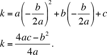
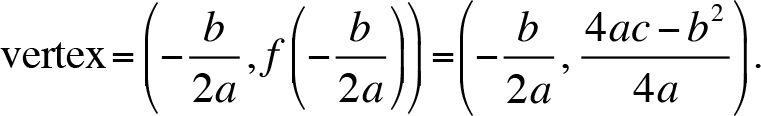
The vertex of the parabola is the lowest point on the graph if the graph opens upward and the highest point on the graph if it opens downward. The parabola is a symmetric figure and the axis of symmetry is x = h where the vertex is (h, k ). Furthermore, 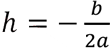for y= ax2 + bx + c . The (h, k ) is a point on y = ax2 + bx +c . So,

k = ah ² + bh +c
.

Thus,

To plot the graphs of quadratic functions, we will follow the subsequent steps.

1. Determine whether the parabola looks up ( a > 0) or looks down ( a < 0).
2. Determine the vertex of the parabola.
3. Find the x -intercept (solving f ( x ) = 0)
4. Find the y -intercept (solving f (0)= c . It is clear that the y –intercept is c .)

Mark the intercepts and vertex in the plane along with an extra check point, if necessary. Connect these points with a smooth curve in the shape of a bowl

Polynomial Inequalities

Up until now, we have discussed the polynomial functions and equalities involving them. We now consider inequalities compromising of polynomials. A statement involving the symbols “>”, “<”, “?”, “?” is called an inequality. In this part we will focus on linear and quadratic inequalities.

We already know that any equation of the form y = ax + b where a ? 0 , is a linear equation. Any of the following inequalities

y > 0, y ? 0, y < 0, and y ? 0,

is called a linear inequality.

For a ? 0 , y = ax ² + bx + c defines a quadratic equation. Any of the following inequalities

y > 0, y < 0, y ? 0, and y ? 0

is called a quadratic inequality.