Statistics 1 Dersi 8. Ünite Özet
Continuous Probability Distributions
Introduction
As it can be recalled that discrete random variables have only a countable number of distinct values such as 0, 1, 2, 3... etc. In other words, a discrete random variable typically comprises of a counting concept. On the other hand, continuous random variables represent entire infinite values in an interval. For that reason, continuous random variables are commonly measured instead of counted.
Continuous Random Variables
A major difference between continuous and discrete random variables is the former takes on uncountable and infinite number of possible outcomes in a given interval. Hence the range of continuous random variable X comprises all real numbers in an interval. random variable X can take unaccountably infinite values. To describe such physical structures through continuous random variables density functions are utilized. Therefore, in contrast to discrete random variables, probabilities in continuous random variables can be determined from the area under probability density function (pdf) which is represented by f (x).
For a continuous random variable X , probability density function f(x) must satisfy the following properties,
(i) f ( x ) ? 0 for all x .
(ii) 
iii)  for all a and b , it is defined the area under probability density function between points a and b .
For a continuous random variable X , for any two points a and b , property (iii) can be written as follows;

Cumulative Distribution Function
Cumulative distribution function (cdf) of a continuous random variable X , denoted by F ( x ) and defined as,
F(x) = P(X ? x) =  , -? < x < ?.
This expression for cumulative distribution function indicates that it’s a cumulative probability value for random variables which are less than or equal to specific random value of x .
Similar to discrete random variables, CDF F(x) of a continuous random variable X, fulfils the following properties.
(i). 0 ? F(x) ? 1 and
(ii). If x 1 ? x 2 then F( x 1 ) ? F ( x 2 )
The major distinction between discrete and continuous CDF, continuous random variable has a continuous CDF, on the other hand discrete random variable has a discrete CDF. Consistent with the definition of CDF, the probability density function of a continuous random variable X can be obtained from the given cumulative distribution function F ( x ) of a random variable X by differentiating. Then for the given CDF F(x),
where the derivative exists.
Mean and Variance of a Continuous Random Variable
The mean of the continuous random variable is denoted by  , the mean is also called as expected value and denoted by E(x) . The variance is denoted by V(x) or
  and it’s a measure of the scattering or variability for data set. The mean and variance can be calculated through these formulas respectively;
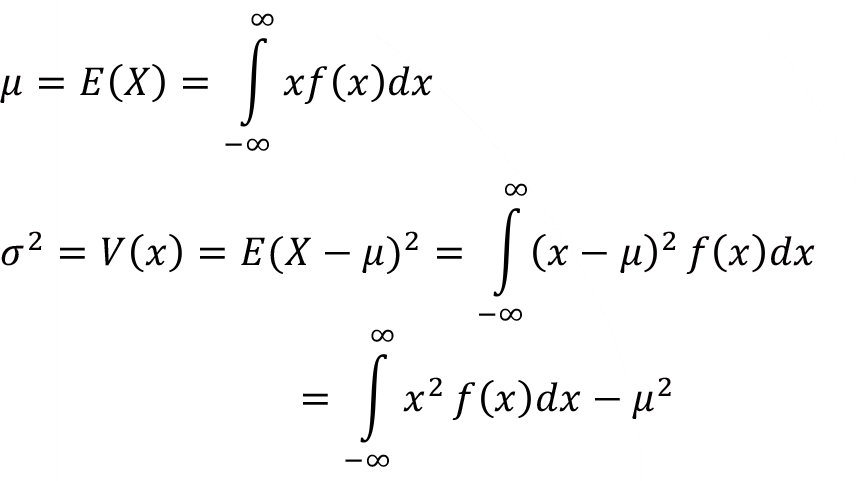
Last term of the variance formulation can be expressed in terms of expected values,
![V(X)=E(X2) -\left [ E(X) \right ]^{2}](https://aofsoru.com/Content/uploads/ozet/8871c08cee38-424c-4525-adfb-6b0ee9e23ac3.gif)
The standard deviation of random variable X is a square root of variance 
Uniform Distribution
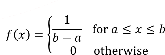
Continuous uniform distribution is the one of the easiest continuous random variables and the probability density function f (x) of the continuous random variable X takes a constant value over the range of the random variable X is defined. Uniform random variable denoted as X ~ U ( a , b ) and probability density function f ( x ) of the continuous uniform random variable between points a and b is defined by,
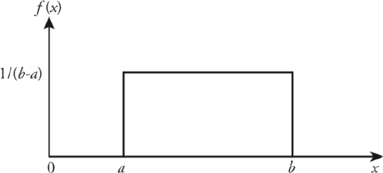
As shown in Figure, the plot of probability density function f ( x ) has a constant value between points a and b . Here point a is the minimum value and the point b is the maximum value of the continuous uniform random variable.
The mean ( ) and variance ( ) of the continuous uniform random variable X between a and b X ~ U (a,b) can be calculated from these formulas,
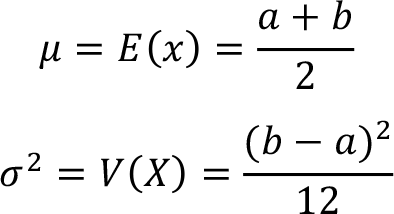
In these mean and variance formulas note that a and b represensts the minimum and maximum values of the random variable X respectively.
Normal Distribution
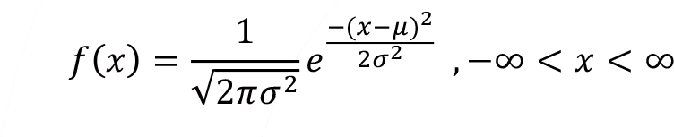
Normal distribution is one of the most significant and extensively used continuous probability distribution. Because of its shape, normal distribution occasionally called “bell curve” or also called “Gaussian curve” which was developed by a mathematician Karl Friedrich Gauss.
Probability density function f ( x ) for the normal random variable X is defined as,
Normal random variable has two parameters,  which defines the center of the continuous probability density function and
  determines the width of the distribution curve. Normally distributed random variable represented using two parameters, and
  , as
, as  . Normal random variable parameters the population mean , defined in the range of -? < < ? and the population standard deviation > 0. In that case mean of a normal random variable can have both positive and negative values including zero. On the other hand, standard deviation of the normal random variable can have only positive values. In the probability density function of the normal random variable, e (Euler number) is irrational mathematical constant approximately equal to 2.71828 and
  number approximately equal to 3.14.
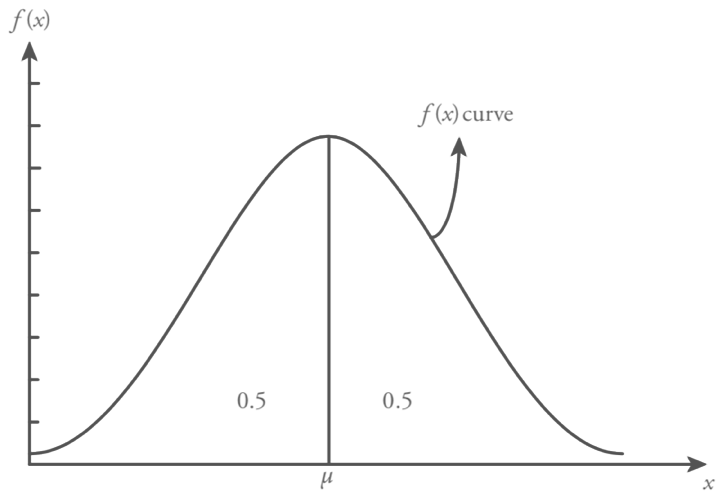
Normal distribution is a symmetric distribution where the random variable values are uniformly scattered around the mean. Figure shows a symmetric distribution, population mean µ, location parameter, defines the center of the normal distribution function and population standard deviation ?, scale parameter, states that the spread (variation) of the distribution function.
Probability density function f ( x ) of normal distribution has the following properties. Clearly The first two of them are common properties for all probability density functions.
(i) f ( x ) ? 0 for all x values.
(ii) 
(iii) The normal distribution function curve is symmetric around the mean, .
(iv) The probability density function f(x) does not the touch and intersect x axis.
The area under the probability density function f(x) for the range of one, two and three standard deviations around the mean covers the 0.683, 0.954 and 0.997 percent of the total area respectively. This handy condition for normal random variable with parameters and is summarized below and also shown in Figure.
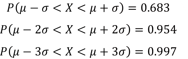
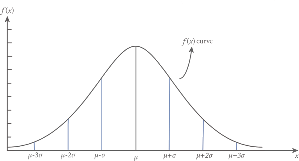
In practice, if the variable that is the interest of the investigation follows a perfect normal distribution then 68.3% of the observation will lie ± 1? of the arithmetic mean, 95.4% of the observation will lie ± 2? of the arithmetic mean and 99.7% of the observation will lie ± 3? of the arithmetic mean.
Standard normal distribution is a special case for the normal distribution where the mean = 0 and the standard deviation = 1 of the distribution. Standard normal variable denoted as z ~ N (0,1).
Every normal distribution can be standardized by using the following formula

Using this simple formula, every normal distribution may be transformed in to standardized normal distribution. Every data point in the normal distribution will get a one to one corresponding value of z .
Table 8.1 gives the cumulative distribution function values of the standard normal distribution in the way that  . The Table 8.1 creates an opportunity for a researcher to calculate all possible probabilities related with a normal distribution once the arithmetic mean and the standard deviation of the distribution had calculated.
(Check Statistics 1 book, page 193, for the Table 8.1)
The Standard Normal Distribution
Probability density function f(z) for the standard normal random variable z can be obtained as follows where the mean = 0, the standard deviation = 1 are placed in the normal density function of f(x) . In Figure standard normal distribution f(z) is shown.
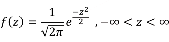
standard normal curve is symmetric around the mean µ = 0. The area under the standard normal distribution is equal to 1 and equally distributed on both sides of the mean µ = 0. Additionally, for the standard normal distribution the values on the horizontal axis are called z values or z score. To obtain the probability values for the standard normal distribution, we utilize the Table 8.1. In this table the area under the standard normal distribution from z = 0 to z = 3.99 are presented. In this table the given probability values are f (z) curve -3 -2 -1 µ=0 1 2 3 z Figure 8.9 Standard normal distribution function between z = 0 and positive z values (z > 0) which include the right-hand side of the distribution function. Nevertheless, due to the symmetry of the standard normal distribution around mean µ=0, the probability values between z=0 and negative z values (z<0) are equal to values on the right-hand side of the standard normal curve. Therefore, the given table values from z=0 to positive z values (z>0) are also usable for the values from z = 0 to negative z values (z>0).
Example:
Consider a standard normal variable and calculate the following probabilities through the standard normal table (Table 8.1).
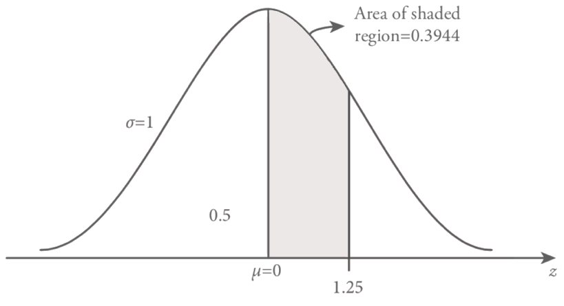
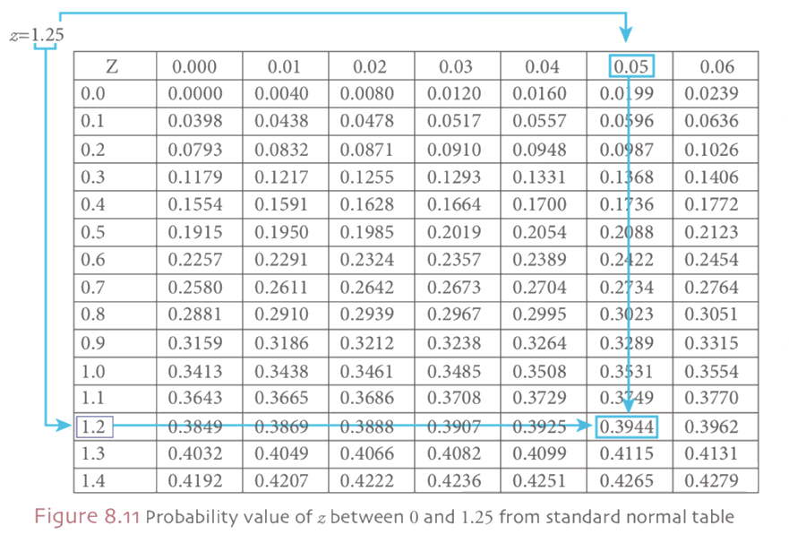
Find the probability of z between 0 and 1.25
The probability of z between 0 and 1.25, under the standard normal curve is the shaded area which is shown in the Figure 8.10. To find the probability value of z between 0 and 1.25 we resort to Table 8.1, standard normal table. Figure visualize that how to obtain the probability value of the required area under the standard normal curve. As it’s shown in Figure 8.11 to find the probability value of z between 0 and 1.25, first reading value of 1.2 under z column. Then choose the second digit after decimal point, 0.05 on the right side of the z value row. As a final point, the intersection of the selected column (1.2) and row value (0.05) forms the value of z = 1.25 and the area under the standard normal curve is 0.3944. Therefore, by using the standard normal distribution table we obtain the value of z = 1.25, then;

probability of obtaining a value of z between 0 and 1.25 is equal to 0.3944.
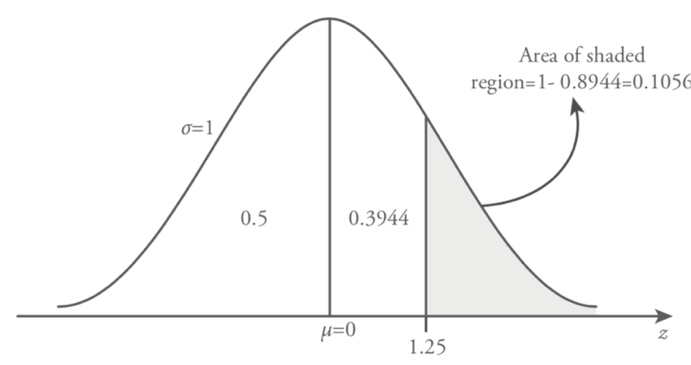
Find the probability that P( z > 1.25 ) .
The given probability question that we consider is the right side of the z=1.25 value. As we stated earlier in this section standard normal distribution table (Table 8.1) provides the probability values between mean (0) and z . Therefore, in order to calculate the necessary probability value, we need to subtract P ( z > 1.25 ) from 1. Because of the symmetry of the standard normal curve the total area on the left side of the z = 0 is 0.5 and we already obtained the value of z between 0 and 1.25, P( 0 ? z ? 1.25 )= 0.3944 . Consequently, the probability in the question can be calculated as follows,


Example:
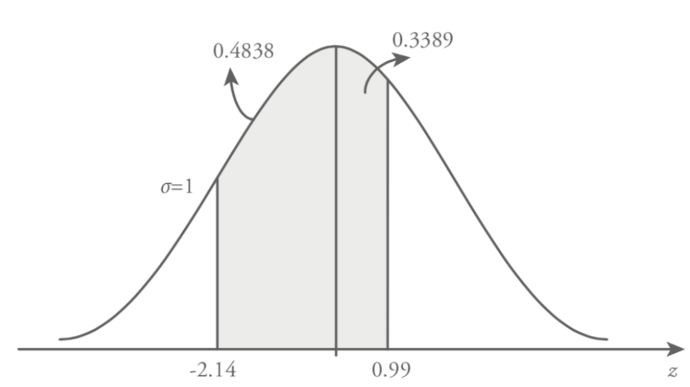
Consider the distribution of a variable is standard normal and find the following probability, P (-2.14 < z < 0.99)
In this example the examined area is shown in Figure 8.17. To find the shaded area under standard normal curve between z = -2.14 and z = 0.99, we will find area of two shaded regions. In this case the area of shaded region examined under two parts, the first one is between z = -2.14 and z = 0 and the second one is between z = 0 and z = 0.99.
The first part of the shaded area is between z = -2.14 and z = 0. As it’s specified previously, stated normal distribution is symmetric around the mean µ = 0. Hence, the area under standard normal curve between z = -2.14 and z=0 equal to the area between z = 0 and z = 2.14. To find the area between z = 0 and z = 2.14 we utilize the standard normal table (Table 8.1). This probability value is obtained from Table 8.1, first we find the value of 2.1 under z column and then choose the second digit after decimal point, 0.04 on the right side of the z value row. The intersection of the selected column (2.1) and row value (0.04) forms the value of z = 2.14 and the area under the standard normal curve is 0.4838.
The second part of the shaded area is between z = 0 and z = 0.99. From the Table 8.1 we find the value of z = 0.99 in a similar manner as defined earlier.
P (-2.14 < z < 0 ) = 0.4838
P ( 0 < z < 0.99 ) = 0.3389
Therefore, the whole area of the shaded region is the total of these two areas under the standard normal curve, namely;
P ( -2.14 < z < 0.99 ) = 0.4838 + 0.3389 = 0.8227
Normal Distribution Applications
Any normal distribution random variable to a standard normal distribution random variable through the following operation;
In this transformation formula Z and X represents the standard normal and normal random variable respectively. Also, mean and standard deviation of the normal random variable is represented by and .
Example:
Assume that in a supermarket checkout lane the total service time is normally distributed with a mean of 260 seconds and a variance of 156.25 seconds. Find the probability that a randomly selected customer’s service time is longer than 280 seconds. The random variable X represents the service time for the checkout lane which is normally distributed with a mean of 260 seconds and a variance of 156.25 seconds. In other words, the standard deviation of the service time is = 156.25 = 12.5 and X ~ N (260, 12.5).
The required probability in this question is a randomly selected customer’s service time is longer than 280 seconds, P ( X > 280) . This circumstance is shown in Figure
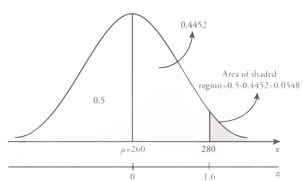
The given probability question that we consider is the right side of the z=1.6 value. As we stated earlier in this section standard normal table (Table 8.1) provides the probability values for the Z values between 0 and z, P ( 0 ? Z ? z ) . Also because of the symmetry of the standard normal distribution the area on the right side of the z=0 is 0.5. Therefore, to calculate the necessary probability value we need to subtract P (Z > 1.6) from 0.5. Consequently,
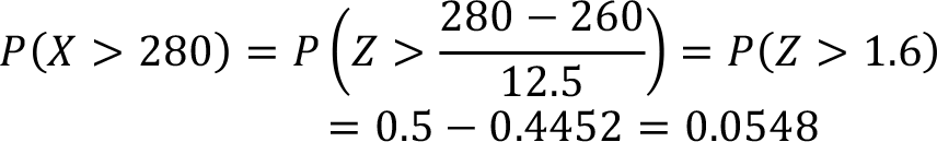
Hence the probability that a randomly selected customer’s service time is longer than 280 seconds is 0.548.
Exponential Distribution
Exponential distribution is another most significant and extensively used continuous probability distribution. Exponential random variable is frequently used to model the time interval between two events.
Exponential random variable is defined with a parameter ? and its represented as X~Exponential (?). In that sense the exponential random variable X defines the time interval between two consecutive events of a Poisson process with a mean of µ = ?. Here ? parameter defines the number of events is a certain time period.
The probability density function of exponential random variable X is as follows,
Here, e (Euler number) is irrational mathematical constant approximately equal to 2.71828,  is the mean number of outcome occurrences in a unit time interval.
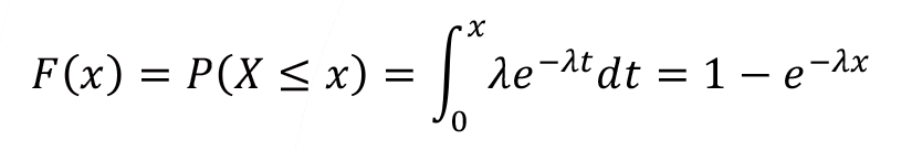
The cumulative distribution function of the exponential distribution of X can obtain through the definition of the cumulative distribution function.
The mean ( ) and variance (  ) for exponential random variable
  with parameter can be calculated from these formulas,
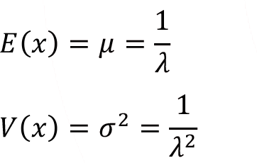
Hence from above given formula it’s clear that the mean and the standard deviation of the exponential distribution are equal.
Example:
Failure time of a certain part of a machine can be modelled by an exponential distribution with a mean of 4000 hours. Find the probability that the machine part will run at most 5000 hours.
In this problem exponential random variable X represents the time to failure of the machine part. Also, since the mean of the failure time is exponential random variable,
The probability density function is as follows,

Therefore  and to find the probability of the machine part will run or function at most 5000 hours.
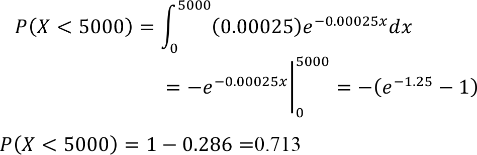
Therefore, the probability that the machine part will run at most 5000 hours is 0.713.
-
Çıkmış Soruları Gönder Para Kazan!
date_range 2 Temmuz 2026 Perşembe comment 25 visibility 4664
-
2025-2026 Öğretim Yılı Yaz Okulu Kayıt Duyurusu
date_range 29 Haziran 2026 Pazartesi comment 4 visibility 977
-
2025-2026 Öğretim Yılı Bahar Dönemi Dönem Sonu (Final) Sınavı Sonuçları Açıklandı!
date_range 18 Mayıs 2026 Pazartesi comment 1 visibility 3155
-
AÖF 2025-2026 Öğretim Yılı Bahar Dönemi Dönem Sonu Sınavı sorularına itiraz
date_range 12 Mayıs 2026 Salı comment 1 visibility 1354
-
2025-2026 Bahar Dönemi Dönem Sonu (Final) Sınavı Sınav Bilgilendirmesi
date_range 4 Mayıs 2026 Pazartesi comment 2 visibility 3293
-
Başarı notu nedir, nasıl hesaplanıyor? Görüntüleme : 28037
-
Bütünleme sınavı neden yapılmamaktadır? Görüntüleme : 16403
-
Harf notlarının anlamları nedir? Görüntüleme : 14808
-
Akademik durum neyi ifade ediyor? Görüntüleme : 13935
-
Akademik yetersizlik uyarısı ne anlama gelmektedir? Görüntüleme : 11855