Statistics 1 Dersi 7. Ünite Özet

Discrete Probability Distributions

Özet

Introduction

The major distinction between relative frequency distributions and probability distributions is the concept of the random variable. In this respect, response variable of the frequency distribution is equal to the random variable of the probability distribution. A random variable is a unique numerical value whose possible values are results within the sample space of a probability experiment. There are two types of random variables discrete and continuous.

Probability Distributions

Each event in a random experiment can be assigned a value where it will be the value of the random variable under consideration. Therefore, a random variable carries a unique numerical value which is determined by random probability experiment and its associated outcomes in the sample space. In statistical notation random variables represented by capital letters such as X, Y and so on. For example, if a coin is tossed, a random variable X represents the outcomes of the random experiment, namely head (H)or tail (T). Discrete random variables have only a countable number of separate values such as 0, 1, 2, 3... etc. Conversely, continuous random variable can take entire infinite values in a given interval. Because of this reason, continuous random variables are commonly measured instead of counted.

The probability distribution of a discrete random variable is a list of odds associated with each of its possible values. It is also called the probability function or the probability mass function. Basically, we can define probability function as a rule that assigns probabilities to the values of random variables. For a discrete random variable X, probability function (probability mass function) must satisfy the following properties,

The probability of each value of the discrete random variable X must be between or equal to 0 and 1.

(i). $0\leq P(X=x)\leq 1$ for all x

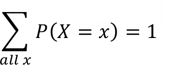
(ii). The sum of the probabilities of each outcome of the random variable must equal 1.

Cumulative Distribution Function

Cumulative distribution function (CDF) of a discrete random variable X, denoted by F (x) and defined as,

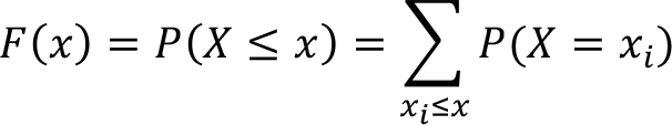
This expression for cumulative distribution function implies that it’s a cumulative probability value for random variables which are less than or equal to specific random value of x _i .

For a discrete random variable X , CDF F(x) fulfills the following properties.

(i). 0 ? F(x) ? 1 and

(ii). If x ₁ ? x ₂ then F(x ₁ ) ? F(X ₂ )

Arithmetic Mean and Variance of a Discrete Random Variable

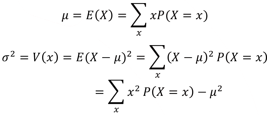
The arithmetic mean of the discrete random variable is denoted by µ, the mean is also called as expected value and denoted by E (x). The variance is denoted by V (x) or ?2 and it’s a measure of the scatter around arithmetic mean or variability for a data set.

The arithmetic mean, and variance can be calculated using the following equations, respectively;

The standard deviation of random variable X is a square root of the variance $\sigma =\sqrt{\sigma ^{2}}$

It is clear that from the above equation the arithmetic mean of a discrete random variable X is weighted value through the possible value of the random variable and associated probability. Also, the variance of a discrete random variable X is all squared deviations are weighted with related probability.

Example: Three coins are flipped, and the random variable X is the number of tails in this experiment. Let’s calculate the arithmetic mean µ and variance ?2 of this discrete probability function. First, we’ll calculate the arithmetic mean of random variable X,

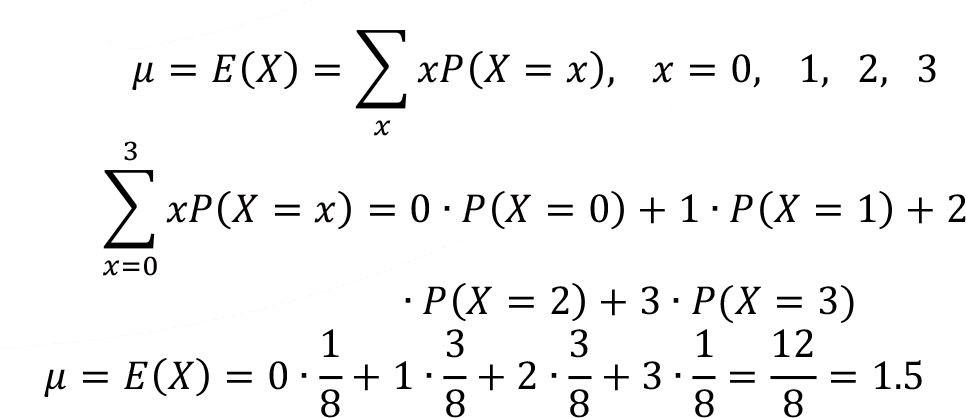
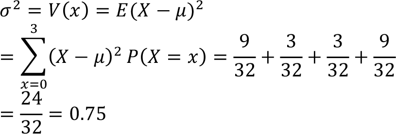
In this example, the calculated arithmetic mean is µ = 1.5; this means that if we repeat this experiment many times, we’ll observe the theoretical value of arithmetic mean 1.5. Variance of the same problem is then

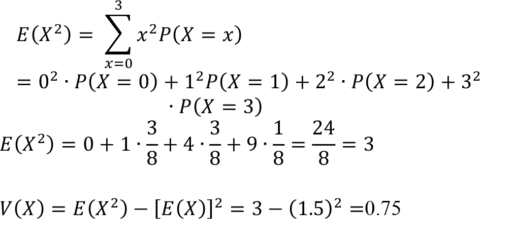
Or using the second approach

Binomial Distribution

Binomial distribution is a widely employed discrete probability distribution in statistics where a set of independent observations constitutes exactly two disjoint outcomes of a trial. Therefore, in binomial distribution, an outcome of a random experiment can be classified under two different categories. For example, when a die is tossed once we observe six different numbers, that is x = 1, 2, 3, 4, 5 and 6. If we classified these outcomes as even or odd numbers then we will get two different outcomes. A random experiment (trial) with only two possible outcomes is frequently used and called a Bernoulli trial with the following properties;

i. Each trial has only two possible outcomes, such as head and tail, 0 and 1 or success and failure.

ii. The trials are independent experiments.

iii. The probability of success, denoted by and the probability of failure, denoted by remains constant for all trials (p + q = 1).

These types of circumstances in random experiments are called binomial experiment and it’s a frequently used discrete probability distribution called Binomial distribution which is the probability distribution for the number of success in a series of Bernoulli trials.

Binomial random variable represented as X ~ Binomial (n,p) . The probability mass function of random variable X is;

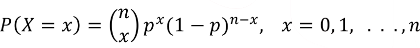
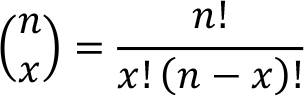
Where $(_{x}^{n})$ is the binomial coefficient and it’s a positive integer. The binomial coefficient is calculated by using the following formula,

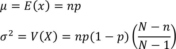
The mean ( $\mu$ ) and variance ( $\sigma$ ² ) of the binomial random variable X ~ Binomial (n,p) can be calculated from these formulas

$\mu$ = E (x) =np and

$\sigma$ ^{2 = V (X) = np (1 - p )}

Example:

Consider the example 7.3, where 3 coins flipped simultaneously and observed number of tails as a random variable in this experiment. In this example random variable X comply with the binomial random variable properties.

$X \sim Binomial(n=3,p=\frac{1}{2})$

Then we calculate following probabilities through binomial distribution. Determine the probability of getting two tails when three coins are flipped simultaneously.

Here random variable X represents the number of tails,

$p(X=2)=(_{2}^{3})(_{2}^{1})^{2}(_{2}^{1})=\frac{3!}{2!1!}(\frac{1}{4})(\frac{1}{2})=\frac{3}{8}$

The probability of getting 2 tails when 3 coins are flipped is 3 / 8.

Determine the probability of getting at least two tails when three coins are tossed.

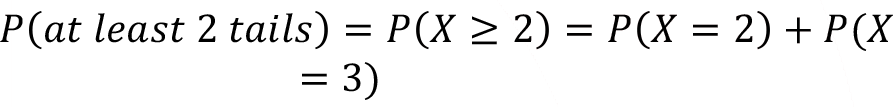
To obtain this probability we will calculate P (X= 2) and P (X = 3) separately.

$P(X=2)=\frac{3}{8}$

$P(X=3)=(_{3}^{3})(_{2}^{1})^{3}(_{2}^{1})^{0}=1(_{8}^{1})=\frac{1}{8}$

$P(X\geq 2)=P(X=2)+P(X=3)=\frac{3}{8}+\frac{1}{8}=\frac{4}{8}=\frac{1}{2}$

Poisson Distribution

The Poisson distribution is widely used for discrete probability distribution which is used to model the number of outcomes occurring during a specified time interval or in a definite region. Here, the time interval indicates any length, for instance an hour, a day, or a month. Also, the definite region term means that a piece of line segment, an acre, size of a football field, a volume.

Some illustrations of random variables that generally conform to model by means of Poisson distribution are presented below.

The number of customers served by automated teller machine in a day.
The number of telephone calls received by a technical support center in a week.
The number of newspapers sold on a particular day. The Poisson distribution has the following properties,

a. The number of outcomes occurring in one-time interval is independent of the number of occurrences in other disjoint time intervals.

b. The probability of the event occurring in one-time interval or definite size region is same for each identical time interval or region. Moreover, it’s assumed that average number of events in a unit time proportional to the length of time. For instance, if it is given 4 Poisson events occur in an hour, this information means that 2 Poisson events occur in 30 minutes and 48 Poisson events occur in 12 hours’ time period.

c. The probability of more than one outcome occurrence in a short time subinterval is zero or insignificant.

The random variable X that equals the number of outcome occurrence in the time interval is a Poisson random variable with parameter $\lambda$ > 0 and represented as X ~ Poisson ( $\lambda$ ) . The probability mass function of random variable X is;

$P(X=x)=\frac{e^{-\lambda }\lambda ^{x}}{x'}, x=0,1,2, ... , and\lambda > 0$

Here, e (Euler number) is irrational mathematical constant approximately equal to 2.71828, $\lambda$ is the mean number of outcome occurrences in a unit time interval.

The mean ( $\mu$ ) and variance ( $\sigma ^{2}$ ) of a Poisson random variable X ~ Poisson ( $\lambda$ ) with parameter $\lambda$ can be calculated using the following formulas,

$\mu =E(x)=\lambda$

$\sigma ^{2}=V(X)=\lambda$

As it’s indicated in the properties of Poisson distribution, it’s essential to use consistent time or region units in the determination of probabilities, mean, and variance with the Poisson random variable.

Example:

A call center of a bank receives, on average, 6 calls per hour and number of calls follows a Poisson distribution.

Determine the probability of exactly 5 calls in an hour. In this question the random variable X represents the number of calls per hour received by the call center.

Then $X\sim Poisson(\lambda =6)$

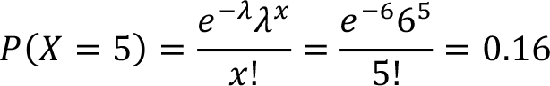
Therefore, the probability exactly 5 calls per hour is 0.16 in this call center.

Determine the probability of receiving at least 4 calls in an hour. In this question the expression ‘at least 4 calls’ specifies four or more calls per hour. In this condition it’s easier to find the probability of 0, 1, 2 and 3 calls then subtract this sum of the probabilities from total 1 to get the probability of at least 4 calls per hour.

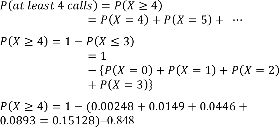
Therefore, the probability of receiving at least 4 calls in an hour is 0.848.

Hypergeometric Distribution

Previously, in section 7.3, we examined binomial distribution, and its principal assumptions are n independent trials with two possible outcomes (success or failure) for each trial, and the success probability remains constant for each trial. Therefore, in binomial distribution the sampling process is carried out with replacement. On the other hand, hypergeometric distribution doesn’t involve with independence assumption for each trial and accordingly the sampling process is established on without replacement. Because of these features, hypergeometric distribution is broadly used in various real-life applications especially for acceptance sampling in quality control.

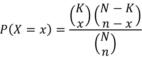
Hypergeometric random variable X is the number of observed items which are categorized as success and represented as X ~ Hypergeometric( N, K, n) . The probability mass function of random variable X is;

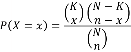, where max (0,n + K - N )

$\leq x\leq min(K,n),K\leq N and n\leq N$

Where $(_{x}^{K})$ is the binomial coefficient and it’s a positive integer. The binomial coefficient is calculated by using the following formula,

$(_{x}^{K})=\frac{K!}{x!(K-x)!}$

Similarly, we can calculate the $(_{n-x}^{N-K})$ and $(_{n}^{N})$ coefficients and obtain the probability of the Hypergeometric random variable X.

In the above given probability distribution function of hypergeometric distribution n represents the number of randomly selected items without replacement from the finite population of size N . Also, a set of N items comprises of K items which are categorized as success and remaining N - K items categorized as failures.

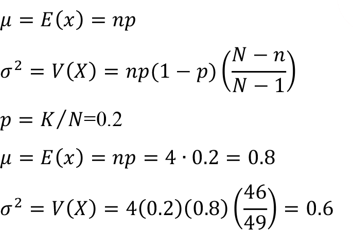
The mean ( $\mu$ ) and the variance ( $\sigma ^{2}$ ) of a hypergeometric random variable X ~ Hypergeometric ( N, K, n ) . with parameters N , n and K can be calculated as follows,

Where p depicts the ratio of success in the population of N items ( p = K / N ).

Example:

Random variable has hypergeometric distribution with parameters N = 50, n = 4 and K = 10.

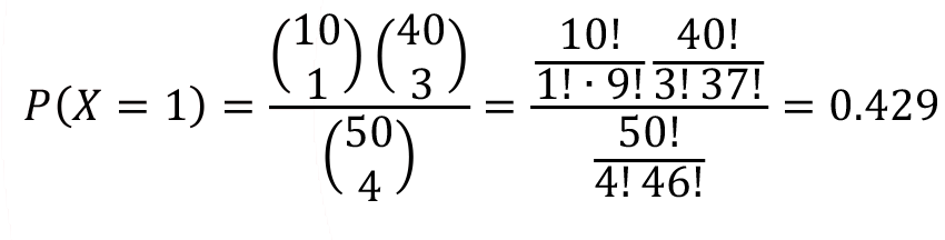
a) Find the probability of random variable X is exactly equal to 1.

b-) Find the probability of random variable X is less than 2.

c) Determine the mean and variance of the random variable X .

a-) N = 50, n = 4 and K = 10

, where max (0, n + K - N )

$\leq x\leq min(K,n),K\leq N and n\leq N$

P(X< 2)=P(X=0)+P(X=1)

$=\frac{(_{0}^{10})(_{4}^{40})}{(_{4}^{50})}+\frac{(_{1}^{10})(_{3}^{40})}{_{4}^{50}}=0.826$

c) The mean ( $\mu$ ) and the variance ( $\sigma ^{2}$ ) of a hypergeometric random variable X ~ Hypergeometric ( N, K, n ) . with parameters N , n and K can be calculated as follows,

PDF YÜKLE PARA KAZAN

Bahar Dönemi Dönem Sonu Sınavı

25 Mayıs 2024 Cumartesi

Duyurular

Aöf Duyuru ve Haberleri

2023-2024 Öğretim Yılı Bahar Dönemi Ara (Vize) Sınavı Sonuçları Açıklandı!
1 Nisan 2024 Pazartesi 3 1869
2023-2024 Bahar Dönemi Ara (Vize) Sınavı Sınav Bilgilendirmesi
20 Mart 2024 Çarşamba 4 2906
2023-2024 Bahar Ara Sınavı Giriş Belgeleri Yayımlandı!
20 Mart 2024 Çarşamba 0 552
Çıkmış Soruları Gönder Para Kazan!
21 Şubat 2024 Çarşamba 2 1087
2023-2024 Bahar Dönemi Ara (Vize) Sınavı İçin Sınav Merkezi Tercihi
6 Şubat 2024 Salı 1 2413

Sıkça Sorulan Sorular

Aöf Hakkında Merak Edilenler

Başarı notu nedir, nasıl hesaplanıyor? Görüntüleme : 24056
Bütünleme sınavı neden yapılmamaktadır? Görüntüleme : 13497
Akademik durum neyi ifade ediyor? Görüntüleme : 11515
Harf notlarının anlamları nedir? Görüntüleme : 11486
Akademik yetersizlik uyarısı ne anlama gelmektedir? Görüntüleme : 9215