Statistics 1 Dersi 6. Ünite Özet

Introduction

Every day we are faced with situations where we have to make decisions that will affect our future life. In many cases, human beings make decisions based on their past experience and knowledge. Unfortunately, in today’s world there are many situations where we have only limited or no information but still have to make some critical choices. Thus, it is important to make use of the data or information that is available. One major approach in these situations is to use probability and statistics. Many of the problems that we are faced can be described by random experiments. Using random experiments to model the problem we are able to use probability theory and also statistics help us make better decisions.

Basic Concepts of Probability

In many situations and applications, it can be seen that a simplified mathematical model can be used to investigate a specific problem at hand. In applications of probability the first step will be to understand and describe the problem by considering all possible outcomes.

Random Experiment

A random experiment is any process that leads to two or more possible outcomes, without knowing exactly which outcome will occur. For example, when a fair die is rolled, we know that one of the six faces will show up but we will not be able to say exactly which face will actually show up. Thus, rolling a fair die is an example of a random experiment.

Note that in a random experiment, although we do not know which outcome will occur, we are able to list or describe all of the possible outcomes.

Sample Space and Events

The set of all possible outcomes of a random experiment is called the sample space. Each possible outcome of a random experiment is called an elementary outcome. Actually, any subset of a sample space is called an event. We say that an event occurs if the random experiment results in one of the basic outcomes of that event.

Let A and B be any two events in a random experiment with sample space S . The intersection of events A and B is the set of all elementary outcomes that belong to both sets. The intersection of two events A and B will be denoted by A ? B . The intersection of two events (A ? B) can be shown as in Figure 6.1. The union of events A and B is the set of all elementary outcomes that belong to at least one of the sets A and B. The union of two events A and B will be denoted by A ? B . The complement of an event A, denoted by A’ or A, is the set of all basic outcomes in S that do not belong to A.

Finding Probability

In order to assign a probability to an event, where an event is a collection of one or more outcomes of an experiment, we may use different approaches. Probability is a value between zero and one, inclusive. Probability describes the relative likelihood an event will occur. In literature, in order to assign probabilities to events there are three known approaches.

Classical Probability

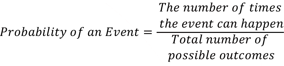
In the classical probability approach to assign a probability to an event, the assumption is that all the outcomes have the same chance of happening. Pick up a six-sided fair die, there are six numbers on each face of the die as 1, 2, 3, 4, 5, and 6. Classical probability says that each side of the die has the same chance to come face up if this die is thrown. Since there are 6 possible outcomes of throwing a six-sided fair die probability of obtaining any number represented on the faces of this sixsided fair die is 1/6. We can formularize this by following equation

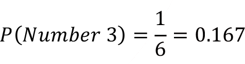
If we go back to six-sided fair die example, if we are interested in probability of a face with number 3 to come up if we throw the die only once, we can easily use classical probability approach. The die is a fair die, that means that all the faces of the die has a same chance to come up if we throw this die, we are only interested in with one outcome which is to observe number 3 on one throw, then the classical probability says that the probability of observing number 3 on one throw is

Empirical Probability

The empirical probability uses the relative frequencies to assign the probabilities to the events. The empirical probability is based on experiments. In order to find the probability of a specific event, the experiments are repeated many times and the observed outcomes of the event we are interested in is counted. We can formularize this by following equation

In Empirical probability, the past information becomes very important. Let’s think a daily life decision that you may make such as buying a watermelon. If you buy the watermelon from the same location over and over, you get a pretty good idea about the quality of the watermelon. So, in your next purchase, you already know your expectations for the quality of the watermelon you may purchase from the same location. As a manager of a company, you may receive particular parts of a product from different suppliers, by keeping good records of the products received for different companies and the number  of faulty products received from each company. When you make your next order from any of these company you may predict the number of faulty products that may come from those companies.

Subjective Probability

In previous approaches to the probability, we have seen some mathematical approaches to assign a probability to an event. Sometimes it may not possible to observe the outcomes of events; therefore, the researcher may assign a probability to an event. In subjective probability approach, the researcher assigns a suitable value as the probability of the event. Therefore, a personal judgement comes in to play to assign the probability. This approach is not favorable method to assign probability, but sometimes if there is no previous knowledge on the subject then the researcher may assign a subjective probability as a starting point. Once enough information about the probability of the event is collected then the researcher may revise this initial subjective probability.

Basic Rules of Probability

Note that in a random experiment the sample space consists of all possible outcomes. We may be able to assign probabilities to the outcomes of a random experiment. When the sample space of a random experiment contains only a finite number of basic outcomes, it is relatively easy to understand and evaluate the probabilities of any event. For example, when rolling two fair dice, finding the probability of any event of this experiment is basically a matter of counting. On the other hand, if the sample space contains infinitely many (countable or uncountable) outcomes, we need to understand the modern concept of probability, which was developed by A. N. Kolmogorov.

The Basic Principle of Counting

Consider any two experiments, of which the first experiment can result in n ₁ and the second can result in n ₂ possible outcomes. Then, considering both experiments together, there are n ₁ .n ₂ possible outcomes. This principle can also be generalized to a finite number of experiments.

In a study about college students, students are classified according to their department and preference of language course. If there are 10 different departments and 5 different language courses, in how many different ways can a student be classified? According to the basic principle of counting, it follows that there are in total 10.5=50 different possible classifications.

When counting the possible outcomes of an event, it is sometimes important to distinguish between ordered and unordered arrangements. When order is important, we call the arrangements of a finite number of distinct objects a permutation.

Considering n distinct objects, there are

n . (n-1) ... 2 . 1 = n!

different permutations of these n objects. In general, if there are n distinct objects, then the number of permutations of size r (1?r?n) from these n objects is denoted by P(n, r) , and is given by

As noted, before if the sample space consists of only a finite number of elementary outcomes, finding the probability of a particular event is basically a matter of counting. On the other hand, if the sample space has infinitely many outcomes, we need to extend the basic ideas of the finite case. This has been established mainly by A. N. Kolmogorov. The most basic properties of a probability function are summarized by the Probability Axioms.

Probability Axioms

Let S denote the sample space of some random experiment. Then

Axiom 1. For any event A?S, P (A )?0.

Axiom 2. P (S )=1.

Axiom 3. Let A ₁ , A ₂ , … be a collection of mutually exclusive events. Then

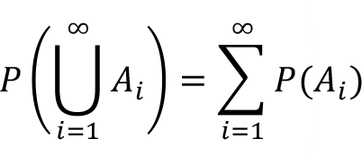
Using these axioms many important rules of probability can be deduced. For example, an immediate consequence of these axioms is that probability is always a number between 0 and 1. That is, if A is any event, then 0 ? P(A) ? 1. Two basic rules that can be obtained from these axioms are as follows:

1) For any event A, P(A) = 1 – P(A)

2) For any two events A and B ,

Example:

A manager in a company has two assistant directors. The probability that the older assistant director comes late to work on a given day is 0.07, whereas for the younger assistant director this probability is 0.05. In addition, the probability that both assistant directors come late to work on given day is 0.03.

What is the probability that at least one of the assistant directors comes late to work on given day?

Define the following events;

O: “The older assistant is late to work.”

Y: “The younger assistant is late to work.”

Then

What is the probability that on a given day one or both assistant directors come late to work?

Note that this event corresponds to

,

and that

Therefore,

Independence and Conditional Probability

When calculating probabilities in some random experiment it is important to know whether the occurrence or non-occurrence of an event affects the occurrence of some particular other event. Consider, for example, two events A and B . We say that events A and B are independent if the occurrence or non-occurrence of event A does not affect the occurrence or non-occurrence of event B .

Sometimes we can use partial information in calculating probabilities. Suppose that we know that event B has occurred, and we are interested in finding the probability of event A . That is, we are interested in finding the probability of A knowing that event B has occurred. This is denoted by P(A/B) and is defined as

assuming that P(B)>0 . Sometimes, it is useful to write this formula in a different form, namely

This formula is actually called the multiplication rule and has important applications.

When the occurrence or non-occurrence of an event A does not affect the occurrence of another event B, then we say that A and B are statistically independent events. This is equivalent to saying that events A and B are statistically independent if and only if

In general, we say that the events A ₁ , A ₂ , …, A _k are mutually statistically independent if and only if

Example:

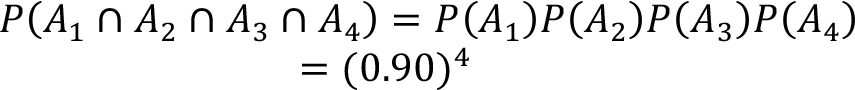
A shop selling mobile phones has purchased four new mobile phones of the same brand and model. It is known that a mobile phone of this brand and model works without any problem for at least 2 years with probability 0.95. What is the probability that all three mobile phones will work without any problem for at least 2 years?

Here, it is natural to assume that a failure of a mobile phone is independent from a failure of another mobile phone. Therefore, if A _i (i =1,2,3,4) denotes the event that the i-th mobile phone will work without any problem for at least 2 years, then the probability is given by

Bayes’ Theorem

An important application of conditional probability is given in the following result, which is known as Bayes’ Theorem.

Let E ₁ , E ₂ , …, E _k be a collection of mutually exclusive and collectively exhaustive events. Then for any event A with P(A)?0 and any i=1, 2…, k

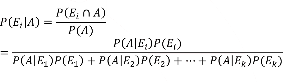
Saying that the events E ₁ , E ₂ , …, E _k are collectively exhaustive means that S = E ₁ ? E ₂ ? ? ? E k.

This theorem enables us to compute a particular conditional probability, such as P(E _i /A) , knowing all the conditional probabilities P(A/E ₁ ), ... , P(A/E _k )

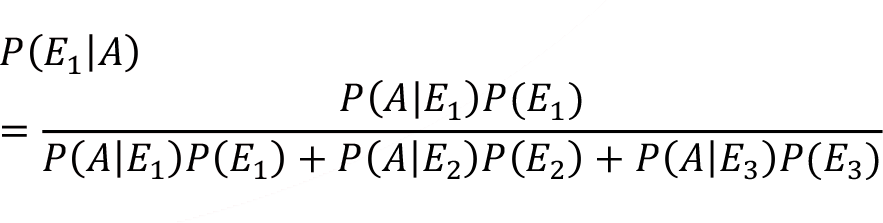
For example, suppose that we know the probabilities of defective items produced by three machines E1, E2, and E3, producing a particular item in some factory. Then, using Bayes’ Theorem, we can find the probability that a defective item is produced by a particular machine, say the first machine. Note that here A denotes an item being defective. Thus, the probability of a defective item being produced by machine one, is given by