Statistics 1 Dersi 5. Ünite Özet

Introduction

The spread of data values in statistics is called variability. Variability measures how close the data points are to each other. In order to study variability, a researcher may look at the distance of observations to the center of data or in an ordered data set, how close data points are to each other in different parts of ordered data. If the data points are very close to the center of the data set such as arithmetic mean, then the variability in this data set will be low for the first case. In the second case when a data set is ordered may be the small values of the data set is closer to each other than the larger values of the same data set.

Range

The range of a data set, shown as R, is the difference between the largest and smallest values and calculated as follows:

R = Largest Value - Smallest Value

Although the range is easy to calculate and to understand, it is generally not a very useful measure of variability. The disadvantage of the range is that it depends only on the highest and lowest observations and it tells us nothing about the variability of the observations which fall between the two extremes.

Variance and Standard Deviation

In order to avoid the disadvantages of the range, we need a measure of variability that is based on including all measurements in a data set. The most important and widely used measure of variability in statistics is the standard deviation.

To determine the variation of a data set in terms of the amounts, we need to measure the deviations from the mean for each observation. Let x ₁ , x ₂ , x ₃ , ... , x _n be a set of measurements constituting a sample, has the mean . The differences x ₁ - , x ₂ - ,  ... , x _n - are called the deviations from the mean.

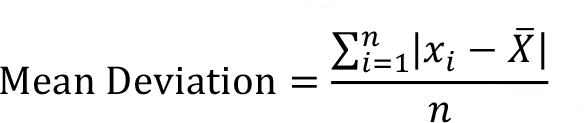
If we sum the deviations from the mean as if they were all positive and divide by n, we obtain the statistical measure which is called mean deviation.

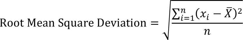
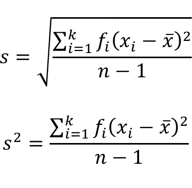
An alternative and more easily interpreted approach is the sum of the squared deviations of the observations from the mean. if we divide the sum of squared deviations by n and take the square root of the result, we get the following equation which is called root mean square deviation.

By modifying this formula by dividing n - 1 instead of n , we get the sample standard deviation, denoted by s. The formula of sample standard deviation is as follows:

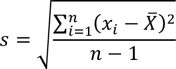
The square of the sample standard deviation is called sample variance.

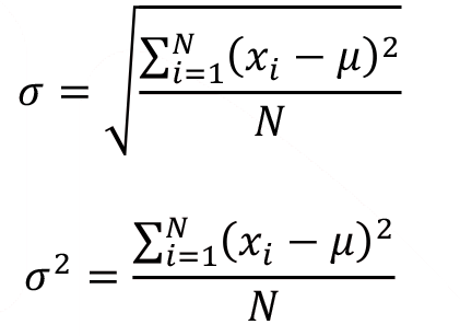
The analogous formulas for the standard deviation and the variance of a population can be obtained by substituting µ for and N for n-1 . The population standard deviation and the population variance are represented by ? (Sigma) and ?2 respectively and calculated as follows.

The sample standard deviation and the sample variance for a frequency distribution can be calculated as follows.

where,

k is the number of classes/categories in the frequency distribution

f _i is the frequency of the ith class/category

x _i is the value of the ith class/category

is the arithmetic mean

n is the total frequency, n =

The sample standard deviation and the sample variance fora grouped frequency distribution can be calculated as follows.

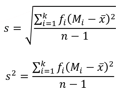
where,

k is the number of classes/categories in the grouped frequency distribution

f _i is the frequency of the i th class/category

M _i is the midpoint of the ith class/category

is the arithmetic mean

n is the total frequency, n =

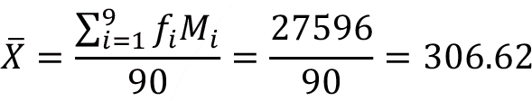
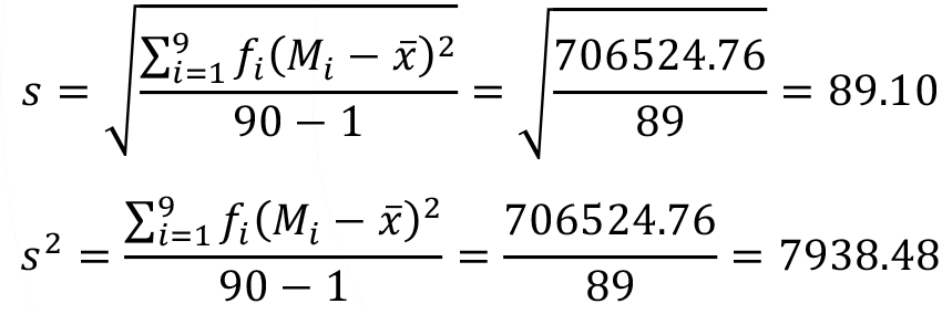
Example: Consider the following grouped frequency distribution of the weekly wages ($). Let’s calculate the sample standard deviation and the sample variance of the data.

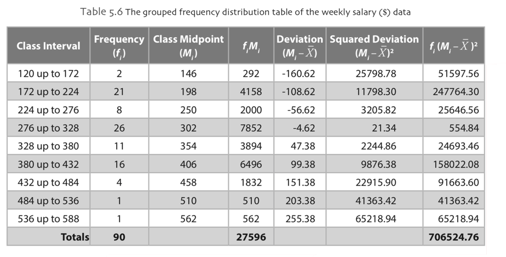
The sample mean of the data, notice that there are 9 classes in this data, is

The sample standard deviation and the sample variance of the data is

Percentiles

How do we measure the variability of different sections of our data, maybe our data is more compact at the upper boundaries then the lower boundaries? Since the standard deviation looks at the overall variability of our data around the mean we need more measures to see the variability in our data.

Another measure of variability includes the use of quantiles or percentiles. First, let’s define the percentiles and their calculations. The percentiles generally are demonstrated as P(m) , where m is the number taking values between 0 and 100. Intuitively, the P(m) percentile of a set of n measurements, arranged in order of magnitude, is the value such m percent of the measurements are less than or equal to that corresponding value.

Some of the specific percentiles frequently used as variability measures are 25th, 50th, and 75th percentiles, often called the first quartile, the second quartile (median), and the third quartile, and denoted by Q1, Q2, and Q3 respectively.

In order to calculate the percentiles, the sample measurements must be sorted in ascending order. Let m indicates the percentile to be calculated. If nm/100=k is an integer, then the P(m) percentile value is the average of the k ^th and (k+1) ^th largest measurements. If k is not an integer, P(m) percentile value is (?k?+1) ^th largest value, where ?k? is the greatest integer function or floor function that gives the largest integer less than or equal to k.

When the data is given as a grouped frequency distribution, the following approximation method can be used to calculate the percentiles.

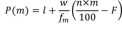
where,

P(m) : percentile of interest

l : lower limit of the interval including the percentile of interest

w : interval width

f _m : frequency of the interval including the percentile of interest

F : cumulative frequency before the interval including the percentile of interest

Example: A real estate agency employs 20 people. The number of years’ experience in the property sector that the employees of the company have is the following.

0, 0, 4, 4, 5, 7, 8, 8, 9, 10, 10, 10, 12, 12, 15, 18, 18, 19, 20, 22

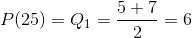
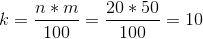
The 25 ^th percentile of the data is calculated as follows.

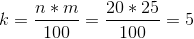
k=5 is an integer, so the 25 ^th percentile is the average of the 5 ^th and 6 ^th largest values.

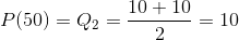
The 50 ^th percentile or the median of the data is calculated as follows.

k=10 is an integer, so the 50 ^th percentile is the average of the 10 ^th and 11 ^th largest values.

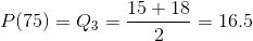
The 75 ^th percentile of the data is calculated as follows.

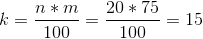
k=15 is an integer, so the 75 ^th percentile is the average of the 15 ^th and 16 ^th largest values.

The 18 ^th percentile of the data is calculated as follows.

k =3.6 is not an integer, so the 18 ^th percentile is P (18) = ( (3.6) + 1) = (3 + 1) = 4 ^th largest value is 4.

Interquartile Range

The second variability measure is the interquartile range (IQR). The interquartile range is the differences between the third and the first quartiles and can be calculated as follows.

The Interquartile range can be thought as the middle 50% of the data, when interquartile range is calculated, we automatically discard the smallest 25% and largest 25% of the data in terms of variability. Therefore, IQR will give us a good indication about the variability of the center data in which the data is sorted from smallest to largest values.

The interquartile range has the advantage over the range of being less compared sensitive to outliers and it is not greatly affected by the sample size. Although IQR has some advantages according to the range, it can be very misleading when the measurements are highly concentrated about the median.

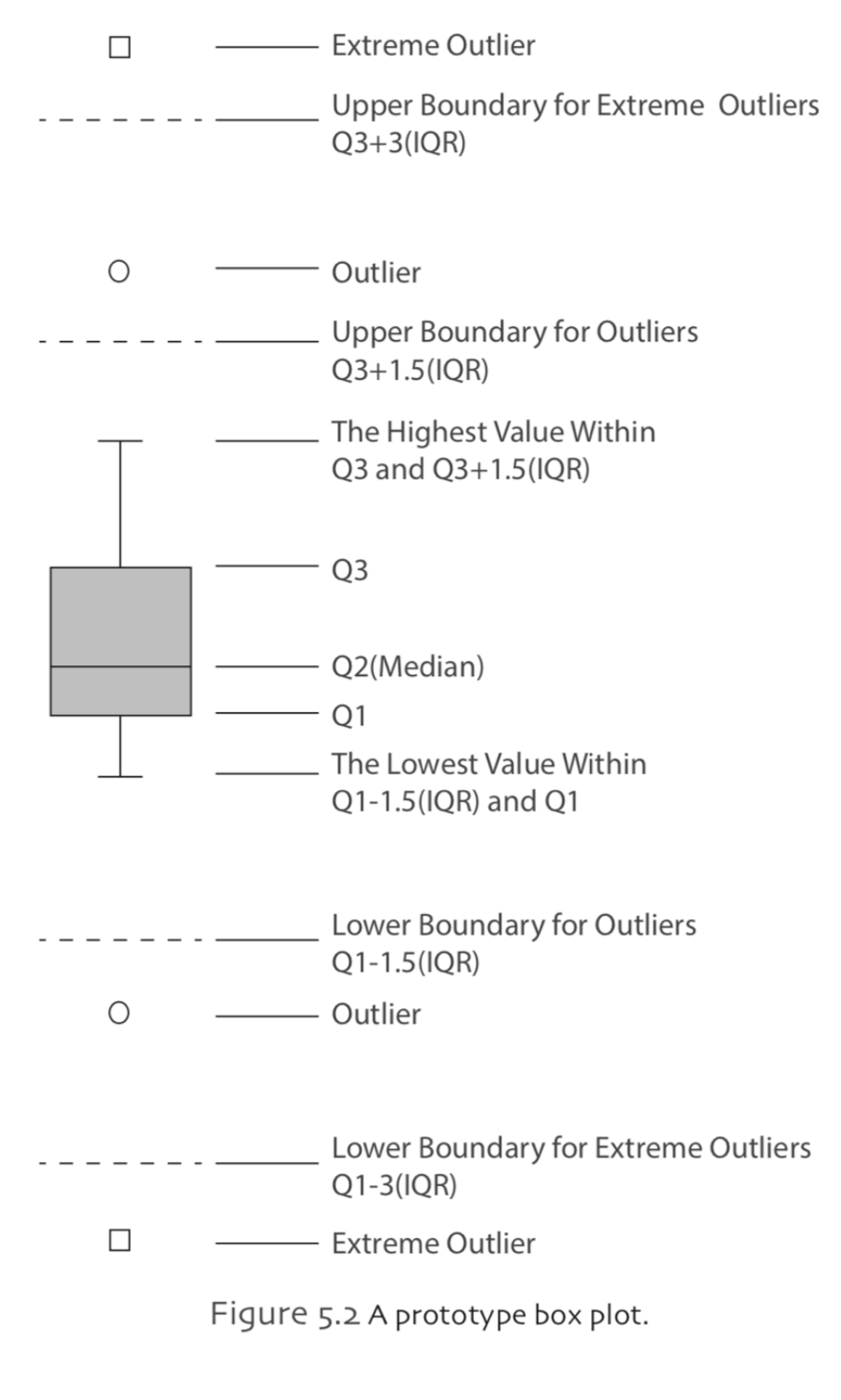
Box Plot

In a box plot, a rectangle (box) with upper and lower edges at the 25th (Q1) and 75th (Q3) percentiles is drawn with a line in the box at the 50th percentile (Q2 ). Lines, which is also called whiskers, are drawn from the box to the highest and lowest values that are within 1.5 x IQR of Q3 and 1.5 x IQR of Q1, respectively. Any observations greater than Q3+1.5 x IQR or less than Q1-1.5 x IQR are plotted individually and called outliers. In the same manner, the observations greater than Q3+3 x IQR or less than Q1-3 x IQR are plotted individually and called extreme outliers.

What information can we obtain from a box plot? The central tendency measure of the distribution is indicated by the median line in the box plot. A measure of the variability of the observations is given by the length of the box. Also, by examining the relative location of the median line, we can obtain about the information of the distribution shape. For instance, if the median line is closer to the 25 ^th percentile than the 75 ^th percentile, there is a greater concentration of observations on the lower side of median and the distribution is right skewed.

A general assessment can be made about the presence of outliers by examining the number of observations classified as outliers and the number classified as extremely outliers.

A prototype box plot is shown in Figure 5.2 as follows.

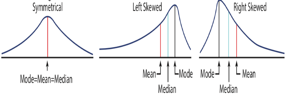
Skewness

A data set which is not symmetrically distributed is called skewed. The mainly observed shapes of distribution are symmetric, left skewed (negatively skewed), and right skewed (positively skewed). If the distribution is unimodal symmetric, the mean, median, and mode are all the same. If the distribution is left skewed, having a long tail in negative direction and a single peak, the mean is pulled in the direction of the tail, and the median falls between the mode and the mean. If the distribution is right skewed, having a long tail in positive direction and a single peak, the mean is pulled in the direction of the tail, and the median falls between the mode and the mean. This information is summarized in Figure 5.4.

Pearson’s Coefficient of Skewness

In the skewed distributions, Karl Pearson showed that the difference between the mean and the mode could be 3 times the difference between the mean and the median. Pearson proposed the following coefficient of skewness.

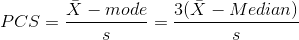
Pearson’s coefficient of skewness (PCS) can take values between -3 and 3. A negative value near -3 shows that the distribution is considerably left skewed and a positive value near 3 shows that the distribution is considerably right skewed. If the PCS is near zero, this indicates that the distribution is symmetric because in this case the mean, the median, and the mode are similar.

Standardized Coefficient of Skewness

Various types of standardized coefficient of skewness (SCS) are used in statistics. The general formula for the standardized coefficient of skewness can be defines as follows.

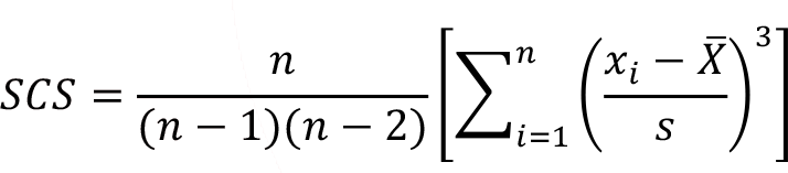
The information on the direction of the difference can be measured. Sum of the cube of the standardizing term over all the values would be near zero, either positive or negative if the data set is symmetric, right skewed or left skewed, respectively.