Statistics 1 Dersi 4. Ünite Özet
Central Tendency Measures
Introduction
Suppose you work as a journalist in the sales department for a newspaper and one day your boss walks into your office and wants to get information about the sales figures of the newspaper for a specific time period. He also would like to learn which columnists are the most followed by readers. What would your best answer be? Of course, you must already have all the data/statistics such as circulations of newspapers in the country, daily sales, popular columnists etc. Well, for the first question, the most reasonable answer you could give would be the average number of newspaper sales in a certain time period. For example, this average is a measure of how many newspapers were sold daily in the last three months. Moreover, you can even provide your boss a chance to compare your newspaper’s sales, giving the average sales of other newspapers in the same time period. For the second question, you simply analyse the reader analytics from your online newspaper and select the most frequently read columnist from the list of all columnists in the paper. So, the basic strategy for answering all these questions, we might want to find the center of data. Such central values are quick and easy ways for a reader to understand the tendency of varied values in an entire data set.
Central Tendency Measures
Central tendency is defined as “the tendency of data to cluster around some random variable value”. The position of the central value is measured by using central tendency measures such as arithmetic mean, median and mode. There are several names used to refer to central tendency in statistics such as “center of the distribution”, “central location”, “representative values”, “central position”, or “measures of location”. There are actually three widely used central tendency measures, namely mode, median, and the arithmetic mean. These measures are different from each other both at the conceptual and computational levels. In general, the mean refers to the average of a set of numbers in the data, the median is the middle value of an ordered dataset, and the mode is the most frequent value in the entire data. The primary purpose of computing them is to determine a single value which may be used to indicate the center of an entire data set including magnitudes of the same data. Another purpose is that since measure of center may represent the whole data, it enables us to make comparisons within or between groups of data.
Mode
The mode is the most common item, observation, or value in a data set which is found by observing the most repeated value. It is also called as a “modal value” that occurs most frequently in a given data. In the following set of observations (3, 1, 3, 2, 10, 9, 3, 10, 3, 4), the mode is 3 because it is the value that occurs most often than any other observation in the data (it is repeated 4 times). Finding a mode for a raw data just involves counting how many times each data value is repeated and finding the highest frequency value. The value with the highest frequency is the mode of the data. Sometimes the data is presented as a grouped frequency distribution, the easiest way to approximate the mode in this case is to identify the class with highest frequency and take the middle of this class as the mode of the grouped frequency distribution. In order to get a better approximation, an interpolation approach can be followed as it is illustrated below by following steps.
You may follow the following steps to calculate the mode of grouped frequency distribution;
Step 1. Create a table of grouped frequency distribution,
Step 2. Identify the highest frequency in your grouped frequency distribution, in Table 4.3 it is equal to 10,
Step 3. Name the class with the highest frequency as modal class, in Table 4.3 the modal class is (15 up to 20),
Step 4. Estimate the mode of the grouped frequency distribution using the following formula,
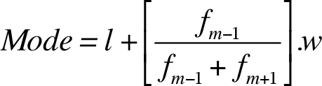
where,
l: lower class boundary (limit) of the modal class
f m-1 : the absolute difference between the frequency of modal class and the frequency of the class preceding (before) the modal class
f m+1 : the absolute difference between the frequency of modal class and the frequency of the class succeeding (after) the modal class
w: class width.
The mode is the main centrality measure for nominal scales (categorical) whereas the mean and the median are not meaningful measures for nominal variables. Besides, the mode can be used with ordinal, interval, and ratio scales. It is also not affected by extreme scores in the data set.
Median
The median of the data set is the value that will be in the middle of the data set when it is ordered from smallest to largest. In general, the median is the value of the variable which divides the total number of objects (total frequency).
In order to find a median value for a raw data, first the data is ordered from smallest to largest. Once the data is ordered, the next step is to identify the location of the median in our ordered data. The location or the position of the median is found by a simple formula; (n + 1)/2. This formula only gives the position of the median in our ordered data and it is important to look at if the number of objects in our data set, n, is an odd number (such as 3, 7, and 9) or an even number (such as 2, 4, and 12). If n is an odd number, the formula will give you a whole number. If there are 7 observations in your data, the formula will give you a result of 4. Therefore, the median of the data is the 4th observation in your ordered data set. Notice that 4 is not the median value but it is the position of your median value. If n is an even number, the formula will give you a decimal number, then the median value is the arithmetic mean of the values in the middle of the data set. If there are 8 observations in your data, the formula will give you a result of 4.5. This means that the median of this data set can be found by the arithmetic mean of the values found by two whole numbers covering this decimal number. Since the result is 4.5, this decimal number is covered by whole numbers 4 and 5, so the arithmetic mean of the 4th and 5th observation in our ordered data is the median value.
In order to find the median value of a frequency distribution, we need to create the cumulative frequency distribution of the data. Once the cumulative frequency distribution is created, the procedure to find the median is the same as in the case of raw data that you have already learned. The cumulative frequency distribution will help you to identify the location or the position of the median value.
Similar to the mode of grouped frequency distribution, the median of the grouped frequency distribution can be calculated by using an interpolation method. In a grouped frequency distribution, first the median class is identified by using (n / 2) formula. Here the formula only helps us to identify where the median value of our data might be, so the formula helps us to find location or position of the median, in this case it will be inside a class, and this class will be called median class. Once the median class is identified the following formula is used to estimate the value of the median:
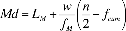
where
L M : Lower boundary (limit) of the class that contains the median (median class)
w : Width of the Median Class (the difference between the lower limit of the class after median class and the lower limit of the median class)
f M : Frequency of the median class
n : The number of observations
f cum : Cumulative frequency of the class preceding (before) median class.
So far, it is clear that the median can be easily detected in a raw data because it represents the middle point of a set of observations. The median can also be estimated by using ogive curve (cumulative frequency polygon). Unlike the arithmetic mean, the median is a robust descriptive statistic because it does not depend on all the values and it retains the position of the data.
The Arithmetic Mean
The arithmetic mean is the most widely used central tendency measure. In daily life, when you hear the word average or mean, it is probably the arithmetic mean of the variable. The Arithmetic mean is generally suitable measure for the variables measured in interval and ratio scales.
Arithmetic Mean of a Raw Data
In order to symbolize the arithmetic mean, two different symbols are used. These symbols are used depending on the type of the data. If the data set, that arithmetic mean is investigated, is a population then the arithmetic mean is symbolized by Greek letter µ (pronounced “mew”), whereas if the data set is a sample then the arithmetic mean is symbolized by  (pronounced “X bar”).
The arithmetic mean of a population is found by using the following formula
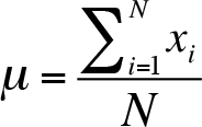
where
x : the value of the individual observation in the population
N : the total number of observations in the population
 : the sum of all values in the population
 : Greek letter for population arithmetic mean
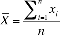
The arithmetic mean of a sample is found by using the following formula
Arithmetic Mean of a Frequency Distribution
The formula of the arithmetic mean for a frequency distribution is adjusted to show every multiplication in each row of the frequency distribution. Using a table, it will be easier to calculate the arithmetic mean of the frequency distribution.
Population arithmetic mean of a frequency distribution is found by using the following formula
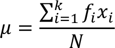
where
x : the value of the individual observation in the population
N : the total number of observations in the population
k : the number of distinct values in the frequency distribution (the number of rows)
 : the sum of all values in the population (frequencies multiplied with observation values)
: Greek letter for population arithmetic mean.
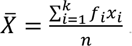
Sample arithmetic mean of a frequency distribution is found by using the following formula
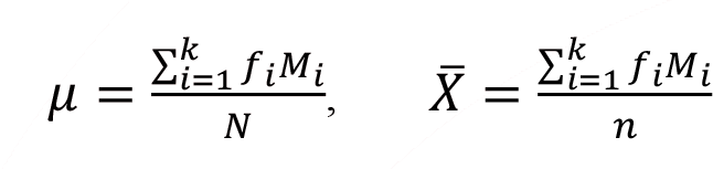
Arithmetic Mean of Grouped Frequency Distribution
Population and sample arithmetic mean formulas for grouped frequency distributions are given as follows, respectively, notice that only difference from the formulas used in frequency distribution is the replacement of x with M (class midpoint);
The Weighted Arithmetic Mean
The weighted arithmetic mean allows a researcher to assign different importance to some of the observations. The relative importance is reflected by using weights. In the case of simple arithmetic mean, each of the data values contribute equally to the final arithmetic mean. In general, the weights cannot be negative numbers, but some weight may be equal to zero. The weighted mean can be calculated using the following equation
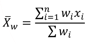
where w is the weight. If you notice that the formula for weighted mean is very similar to the formula of the arithmetic mean of frequency distributions, the only difference now is that the frequencies are replaced with the weights of each row.
Properties of the Arithmetic Mean
Property 1. Suppose that represents the arithmetic mean of a data set, then, If constant value of a is added to each value of this data set, the arithmetic mean of the new data set becomes + a, and similarly; If constant value of a is subtracted from each value of this data set, the arithmetic mean of the new data set becomes - a.
Property 2. Suppose that represents the arithmetic mean of a data set, then, If each value of the data set is multiplied by a constant such as a (a is not equal to zero), the mean of the new data set is a , and similarly, If each value of the data set is divided by a constant such as b (b is not equal to zero), the mean of the new values is /b.
Property 3. For a given data set, the total of the deviations of the values from their arithmetic mean is zero (?(x İ - ) = 0).
Property 4. For a given data set, the sum of the squared deviations of the values from their arithmetic mean is minimum.
Geometric Mean
The geometric mean of the n positive observations x 1 , x 2 , x 3 , ... , x n is the n th root of the product (multiplication) ( x 1 , x 2 , x 3 , ... , x n ). The geometric mean is used when all the observations are positive, this is a limitation of the geometric mean. The following formula can be written for the geometric mean of a data set
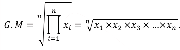
where the Greek symbol  represents the notation for product (multiplication of the values). The geometric mean can be used in many fields, including business (interest rates, proportional growth), communication (aspect ratio of an image), computer science (mindboggling memory), medicine, biology (growth rates), and social sciences (population growth).
Robust Estimators of the Averages
When there are some extreme values (outliers) exist in a dataset, trimmed (truncated) mean and Winsorized mean can be used.
Trimmed (Truncated) Mean
Given a set of observations, x 1 , x 2 , x 3 , ... , x n , n = number of observations, then sort observations, x 1 , x 2 , x 3 , ... , x n , from the smallest to the largest or the largest to the smallest. Trimmed mean involves throwing away a proportion of the outer observations on either side and averaging the remainder. Decide on percentage of the data to throw away, symbolized by p, between 0 and 1, such as 0.20 represents 20% of trimming. Decide how many data points is thrown away, symbolized with k, by using k = np. Throw away the top and bottom (smallest and largest) k observations’ values from the data. Calculate the arithmetic mean of the remaining observations, be careful at this stage, now the number of objects is n – 2k.
Winsorized Mean
The Winsorized mean is similar to the trimmed mean. It was invented by C.P. Winsor (1895-1951). Winsorized mean involves replacing a proportion of the outer observations on either side with the most extreme remaining values and averaging the remainder. In other words, the Winsorized mean can be calculated with the remaining values after replacing a certain number or the proportion of the values at the low and high end of the sorted data. In general, for Winsorized mean, we use 10 to 25 percent of the values of both ends to be replaced.
Given a set of observations, x 1 , x 2 , x 3 , ... , x n , n = number of observations, then sort observations, x 1 , x 2 , x 3 , ... , x n , from the smallest to the largest or the largest to the smallest. Winsorized mean involves replacing a proportion of the outer observations on either side with the most extreme remaining values and averaging the remainder. Decide on percentage of the data to be replaced, symbolized by p , between 0 and 1, such as 0.20 represents 20% of replacement. Decide how many data points is replaced, symbolized with k , by using k = np . Replace the k minimum values with the next smallest observation’s value and replace the k maximum values with the next highest observation’s value. Find the arithmetic mean of the newly created data, now extremes are replaced with most extremes of the remaining data without k observations in either end, therefore number of objects is now equal to n .
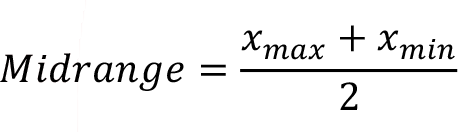
Midrange
Midrange is an arithmetic mean of the extremes in both end of the data set. It only needs the smallest value and the largest value to be given. The arithmetic mean of these two extremes called mid-range. As you remember, the range is the difference between the largest and the smallest values in a set of data. Instead of taking the difference of both ends (range), the average of these numbers is found in midrange. The midrange can be calculated using the following formula
The Usage of The Arithmetic Mean, Median and Mode in Real Life
As mentioned earlier, the mode can be computed for categorical (nominal and ordinal) or quantitative (interval and ratio) data. On the other hand, for the nominal data, the median and the arithmetic mean cannot be used. Median can be a useful measure of location for data measured in ordinal, interval, and ratio levels. The mean can only be computed for the data measured in interval and ratio levels. Even though an arithmetic mean is reported for numerical ordinal data (e.g., Likert scales) in research, there is not a consensus among scientists about whether the arithmetic mean can be used with data measured in ordinal level.
The mode is the simplest, but it is the weakest measure of center. If all values have the same frequency, there is no mode in the data or if two or more values occur with the same frequency, there is multiple modes.
The median is a more useful measure since it represents a more typical score and many people can easily understand it. The mean is a more valid measure of center because it takes into account all the values in a dataset. For this reason, the mean is the most powerful and preferred measure of central tendency in many disciplines.
In bell-shape, unimodal, or symmetric distributions such as normal curve, the mean, median (Md), and mode (Mo) are all equal. In symmetric distributions like bell-shape and rectangular (or uniform) ones, the mean and median are the same value.
When there are extreme values (outliers) in a data set, geometric mean, trimmed mean, Winsorized mean, and the median can be preferred because they are resistant to change from a wild swing in a single observation. For example, if you wish to find the average score of a basketball player in a season, the player may show an extreme performance in one or two games and it affects the arithmetic mean. In such a case the mean would show a much higher value because of one high score. Generally, a good player may have an approximately 20 points average in a 30-game season. However, Erman Kunter a former Turkish professional basketball player for Fenerbahçe scored 153 points of his team’s 175 points against Hilalspor in 1988. This extraordinary performance in one game increases his points-per-game average dramatically. In this case, the median or the trimmed mean would be more appropriate measure compared to the arithmetic mean.
The mean is generally the most proper measure to use when the distribution is continuous and symmetrical, such as normally distributed data. The mean is also the most appropriate one to further statistical applications, especially for inferential purposes. However, for strongly skewed distributions, the median is the most representative one, especially for descriptive analysis. The mode is the most representative measure in nominal level data. For unimodal distributions, the mode, median, and mean would be equal. Overall, it all depends on what you are trying to show in a given data set.
-
Çıkmış Soruları Gönder Para Kazan!
date_range 2 Temmuz 2026 Perşembe comment 25 visibility 4664
-
2025-2026 Öğretim Yılı Yaz Okulu Kayıt Duyurusu
date_range 29 Haziran 2026 Pazartesi comment 4 visibility 977
-
2025-2026 Öğretim Yılı Bahar Dönemi Dönem Sonu (Final) Sınavı Sonuçları Açıklandı!
date_range 18 Mayıs 2026 Pazartesi comment 1 visibility 3155
-
AÖF 2025-2026 Öğretim Yılı Bahar Dönemi Dönem Sonu Sınavı sorularına itiraz
date_range 12 Mayıs 2026 Salı comment 1 visibility 1354
-
2025-2026 Bahar Dönemi Dönem Sonu (Final) Sınavı Sınav Bilgilendirmesi
date_range 4 Mayıs 2026 Pazartesi comment 2 visibility 3293
-
Başarı notu nedir, nasıl hesaplanıyor? Görüntüleme : 28037
-
Bütünleme sınavı neden yapılmamaktadır? Görüntüleme : 16403
-
Harf notlarının anlamları nedir? Görüntüleme : 14808
-
Akademik durum neyi ifade ediyor? Görüntüleme : 13935
-
Akademik yetersizlik uyarısı ne anlama gelmektedir? Görüntüleme : 11855